After downloading the workshop Jupyter notebook, you can upload it to Google Colab to get a quick start, but you will not be able to see the animations.
Overview
Machine Learning and Optimization Seminar
The goal of the Machine Learning and Optimization seminar this year is to expose the participants to topics in machine learning and optimization by:
Facilitating hands-on workshops and group discussions to explore and gain experience
Inviting speakers to introduce machine learning and optimization concepts
We are excited to get started on this but recognize that since neither machine learning nor optimization are standardized in the department, participants will have a varied level of exposure to different topics. Our hope is that we can use this disparity of experience to increase collaboration during the workshops in a way that can’t be achieved during the talks. All are encouraged to share their knowledge and experience with one another openly during the workshops and to give feedback to the organizers after.
All workshop material will be available here for later reference.
This first workshop is focused on tooling and the basic concepts of machine learning and optimization with the goal that everyone can be on the same footing for later workshops.
Your Python environment
It is safe to say that Python is the language of choice for machine learning. This interpreted language has a very clear and high-level syntax, is extremely convenient for interactive programming and debugging, and has an enormous user base of enterprises, researchers, and hobbyists who have built an almost infinite collection of open-source packages for every topic. For these three reasons the workshops for this seminar will use Python.
To get started, we will give the basics of the Python programming language. Just kidding! That would take too long. We will instead guide you on how to install Python most conveniently, teach you how to get started learning about Python, and then point you to a curated library of much more high-quality instruction for using Python. A list of some such references as well as documentation for setup and important Python packages can be found in the Appendix here.
Setting up
Tip
If you are looking for the easiest and most immediate way to get going with a Python Jupyter Notebook, check out the Google Colab section.
Note
This section will require use of a terminal emulator for installing and running Python. If you are not familiar with the terminal, check out this quick tutorial to get started.
If you are using a computer with Windows, the terminal instructions may not apply.
Python is installed by default on MacOS and most Linux distributions. However, it can be challenging to navigate between the versions and packages that your operating system uses and those needed for other projects. Thus, there are a variety of version, package, and environment management tools:
Version management: Which version of Python are you using? Can you change versions to run a specific Python program if it requires?
pyenv
conda/mamba
Package management: How can you install the many amazing Python packages people have created?
pip
conda/mamba
Environment management: If you have two projects that require different packages (or different versions of the same package), can you switch which packages are available depending on which project you are working on?
venv
virtualenv
poetry
conda/mamba
many more
The conda package manager is the only one that fills all three roles. It is formally a part of the Anaconda Python distribution which is a favorite in the fields of data science and machine learning. mamba is a newer and faster rewrite used in exactly the same way and which is highly recommended.
The best way to get started with mamba is to install mambaforge. You can find installer downloads for Windows, MacOS, or Linux here.
For Windows, run the .exe file once it is downloaded.
For MacOS and Linux, open a terminal and navigate to the download location:
cd ~/Downloads
Then run the installer as follows:
./Mambaforge-Linux-x86_64.sh
The installer will walk you through a few steps and end by asking if you’d like to “initialize Mambaforge by running conda init?” Answer yes and restart your terminal. This final command will have added conda and mamba to your system $PATH variable, which means it is available to your terminal. Once restarted, run mamba -V to print the version and to verify that the installation worked.
Environments
The idea of a conda/mamba environment is that once an environment is created and activated, all new packages installed will be added to that environment and will be accessible to any Python program run while the environment is active. As an example, let’s create an environment called workshop with a specific version of Python installed. The following will create the environment and install a specific version of python:
mamba create -n workshop python=3.9
Once created, we can list our environments via the command
mamba env list
# conda environments:
#
base                     /home/user/mambaforge
workshop                 /home/user/mambaforge/envs/workshop
Note that there is a “base” environment which is where conda and mamba themselves are installed as well as their dependencies. The best practice is to create an environment for each of your projects to minimize dependency issues (when packages require separate versions of the same package).
To activate our new environment:
mamba activate workshop
Running mamba env list will now show our active environment via an asterisk:
base                     /home/user/mambaforge
workshop              *  /home/user/mambaforge/envs/workshop
Installing packages
Now that we have activated the workshopconda environment, let’s install some common machine learning packages in Python. It is as easy as writing:
This command will search the conda-forge repository of packages and install the most up-to-date versions (the forge in mambaforge).
Tip
Either conda or mamba could be used for all the commands discussed in this section. However, mamba is significantly faster when installing packages.
Now that these packages have been installed, we can easily use them in an interactive ipython prompt (installed with the jupyter package):
ipython
Python 3.9.13 | packaged by conda-forge | (main, May 27 2022, 16:58:50)Type 'copyright', 'credits' or 'license' for more informationIPython 8.4.0 -- An enhanced Interactive Python. Type '?' for help.In [1]: import numpy as npIn [2]: import matplotlib.pyplot as pltIn [3]: x = np.linspace(0,10,100)In [4]: y = np.sin(x)In [5]: plt.plot(x,y); plt.show()
This should plot a simple \(\sin\) curve.
Cleaning up
After we are done using the environment that has our desired version of Python and the needed packages, we can go back to our regular terminal by deactivating the environment:
mamba deactivate workshop
If we have somehow broken our environment and need to remove it:
mamba env remove -n workshop
There are many more commands and functionalities that conda and mamba provide that can be found in the python resources and packages section of the Appendix.
Google Colab
As an alternative to the entire procedure above, you can use an online Jupyter Notebook service hosted by Google called Colab. This service will get you up and running immediately but cannot save your environment between notebooks and has limited functionality to run scripts, save data, view animations, change package versions, etc. Thus, if your notebook requires a package that is not installed by default, you will need to add the installation command in one of the first notebook cells. For example, to install the reservoirpy package, we would write in a notebook cell:
!pip install reservoirpy
In a notebook, the ! denotes a terminal command. The package will now be ready for import and use within the current notebook session:
from reservoirpy.nodes import Input,Reservoir,Ridge
Basic concepts of machine learning
Machine learning is, at its most basic, automated data analysis, usually with the goal of finding patterns or making predictions. The “machines” in this analysis are equations or algorithms and the “learning” is usually some form of parameter selection and/or fitting. Due to the uncertain nature of most data, the majority of these models are probabilistic in nature. In fact, it can be hard to distinguish the methodological lines between what is termed “machine learning” and the field of statistics. However, there are a few important distinctions between the tools, goals, and terminology of the two areas. Today, machine learning has emerged as a broad description of almost any data-driven computing which may or may not include classical descriptive and inferential statistics [1].
At first glance, machine learning can be separated into three main classes:
Supervised learning: Given dependent and independent variable data, train a model which effectively maps the independent variable data to produce the dependent variable data.
Generalized linear models (linear, logistic, etc. regression)
Naive Bayes
Neural networks (most)
Support vector machine (SVM)
Random forests
etc.
Unsupervised learning: Given data, find patterns (no specified output, though there is still a measure of success)
Clustering
Mixture models
Dimensionality reduction
Association rules
etc.
Reinforcement learning: Given input data and desired outcomes, simulate and use the results to update a model to improve the simulation’s ability to achieve those outcomes
Q-learning
SARSA
etc.
There is an enormous amount of current interest in machine learning methods and there is a corresponding amount of high-quality material discussing it. We will end the introduction here and direct you to established textbooks [1–3], NJIT classes (Math 478, Math 678, Math 680, CS 675, CS 677), and online resources (too many to even start listing).
General procedure
In practice, machine learning algorithms often boil down to an optimization problem. To characterize this in a few steps, consider a problem with data \(x\):
Select a model representation \(f\) with parameters \(p\) for the problem: \[
y = f(x;p)
\]
Determine an appropriate objective function \(\mathcal{L}\): \[
\mathcal{L}(f(x;p),x)
\]
Use an optimization method \(\mathcal{O}\) with parameters \(d\) to find parameters \(p\) that minimize or maximize the objective for the model: \[
p^* = \mathcal{O}(\mathcal{L},f,x;d)
\]
In some sense, this is the same procedure used for inverse problems in traditional applied mathematics but with a broader set of models \(f\) that may or may not be based on first-principles understanding of the problem.
Incorporating data
Depending on the class of problem considered (supervised, unsupervised, or reinforcement), there are a variety of choices for models \(f\) and objectives \(\mathcal{L}\). For supervised learning (the most common), the objective is often to predict or generate the output or dependent variable data of some process. For this, data can be separated into three sets:
Training data (\(x\)): used to tune the parameters \(p\)
Validation data (\(x^v\)): used to evaluate the generalization of the model \(f\) to data not in the training set during training
Testing data (\(x^t\)): used to benchmark the predictive or generative ability of the model after training is completed
A first machine learning problem
Note
The code for this problem will require the following packages: numpy, matplotlib, autograd
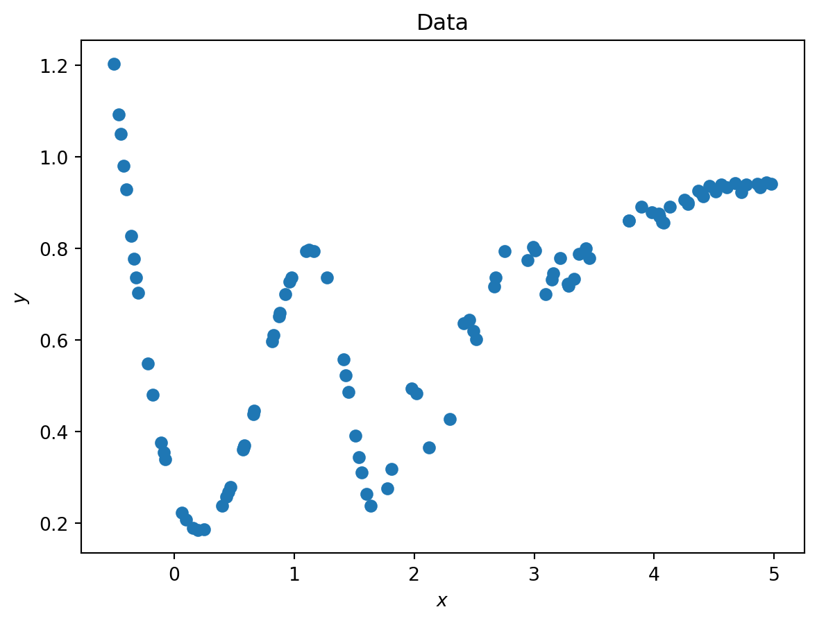
These workshops are about learning by doing, so let’s build understanding by fitting a simple “machine” to some data as a supervised problem. Consider some data \((x,y)\):
Data generation
import numpy as npimport matplotlib.pyplot as plt# To see animations in a Jupyter notebook, uncomment the following line:# %matplotlib notebookdef f_known(x): part1 = np.exp(-x)*(np.sin((x)**3) + np.sin((x)**2) - x) part2 =1/(1+ np.exp(-1*(x-1)))return part1 + part2xsamples = np.random.uniform(-1/2,5,100)ysamples = f_known(xsamples)plt.scatter(xsamples,ysamples)plt.xlabel("$x$"); plt.ylabel("$y$"); plt.title("Data")plt.show()
We would like to fit a model of the following form to this data: \[
f(x;p_0,p_1) = e^{-p_0x}(\sin((p_0x)^3) + \sin((p_0x)^2) - p_0x) + \frac{1}{1 + e^{-p_1(x-1)}}
\]
To formulate this as a machine learning/optimization problem, we can consider an objective/loss to minimize the \(L^2\) norm distance between the model output \(f(x)\) and the true data \(y\): \[
\mathcal{L(f(x;\vec{p}),y)} = ||f(x) - y||_2^2
\] The problem can then be written as the unconstrained optimization problem: \[
p^* = \underset{\vec{p}}{\text{minimize }} \mathcal{L}(f(x;\vec{p}),y)
\] We then expect our model \(f(x;p^*)\) to represent a “machine” that has accurately “learned” the relationship between \(x\) and \(y\).
There are several ways to approach this problem, but a simple and popular approach for a continuous and unconstrained problem is to use an iterative gradient method.
Gradient descent
Gradient descent is a straightforward method taught early in an undergraduate numerical methods class. Its simplicity and relatively low computational cost has made it popular for machine learning methods (which can contain enough parameters that second-order methods, like Newton’s method, are infeasibly expensive because of the Hessian computation). Beginning with an initial parameter guess \(\vec{p}_0\), its update procedure can be written as: \[
\begin{align*}
\vec{p}^{i+1} &= \vec{p}^i + v^i \\
v^i &= -\alpha \nabla_p \mathcal{L}
\end{align*}
\] where \(\alpha\) controls the step size in the direction of the gradient (usually called a “learning rate” in machine learning). This method will follow the gradient of the objective/loss \(\mathcal{L}\) until the objective is sufficiently small, or until it reaches a steady state.
Simply implemented in Python, this method can be written as:
def gradient_descent(f_p,x0,alpha=.2,tol=1e-12,steps=1000): x = x0 xs = [x]for s inrange(steps): v_i =-alpha*f_p(x) xnew = x + v_iif np.linalg.norm(f_p(xnew)) < tol:print("Converged to objective loss gradient below {} in {} steps.".format(tol,s))return x,xselif np.linalg.norm(xnew - x) < tol:print("Converged to steady state of tolerance {} in {} steps.".format(tol,s))return x,xs x = xnew xs.append(x)print("Did not converge after {} steps (tolerance {}).".format(steps,tol))return x,xs
However, this method contains a troublesome parameter \(\alpha\) which, if chosen too large, could prevent convergence of the solution or, if chosen too small, could require an unreasonable number of steps to converge. The method itself is also prone to terminate in local minima rather than in a global minimum unless the correct initial guess and learning rate are chosen. For this reason, “vanilla” (or normal) gradient descent is almost always replaced with a modified method in learning problems [4,5].
The following demonstrates an animation of the above gradient descent method applied to our data with two different learning rates, one successful, one not. It uses the following animation code and the autograd automatic differentiation library that will be further discussed later:
Animation code
from matplotlib import animation as animfrom matplotlib import gridspecfrom mpl_toolkits.mplot3d import Axes3D# To display the animations in a jupyer notebook uncomment the following line:# %matplotlib notebookdef animate_steps_2d(xs,loss,xmin=-.1,xmax=2.5,ymin=-1,ymax=3,interval=50): fig = plt.figure(figsize=(10,6),constrained_layout=True) gs = gridspec.GridSpec(ncols=6,nrows=2,figure=fig) ax = fig.add_subplot(gs[:,0:4],projection="3d") ax1 = fig.add_subplot(gs[0,4:]) ax2 = fig.add_subplot(gs[1,4:]) ax.view_init(47,47) ax.set_xlabel("$p_0$"); ax.set_ylabel("$p_2$"); ax.set_zlabel("loss",rotation=90) ax1.set_xlabel("$p_0$"); ax1.set_ylabel("loss") ax2.set_xlabel("$p_1$"); ax2.set_ylabel("loss") xs_arr = np.array(xs) fxs = np.linspace(xmin,xmax,100) fys = np.linspace(ymin,ymax,100) loss_fx = [loss([fxs[j],xs[0][1]]) for j inrange(len(fxs))] loss_fy = [loss([xs[0][0],fys[j]]) for j inrange(len(fys))] X,Y = np.meshgrid(fxs,fys) Z = np.zeros_like(X)for i inrange(X.shape[0]):for j inrange(X.shape[1]): Z[i,j] = loss([X[i,j],Y[i,j]])# Add surface plot surf = ax.plot_surface(X,Y,Z,cmap="gist_earth") ax1.set_xlim(np.min(X),np.max(X)); ax1.set_ylim(np.min(Z),np.max(Z)) ax2.set_xlim(np.min(Y),np.max(Y)); ax2.set_ylim(np.min(Z),np.max(Z)) plot1 = ax.plot(xs[0][0],xs[0][1],loss(xs[0]),zorder=100,color="red",linestyle="",marker="o")[0] plot2 = ax.plot([],[],[],color="orange")[0]# Add flat plots for perspective plot3 = ax1.plot(fxs,loss_fx)[0] plot4 = ax1.scatter(xs[0][0],loss(xs[0]),color="red",s=100,zorder=100) plot5 = ax2.plot(fys,loss_fy)[0] plot6 = ax2.scatter(xs[0][1],loss(xs[0]),color="red",s=100,zorder=100)def anim_func(i): x_loss = loss(xs[i]) plot1.set_data_3d(xs[i][0],xs[i][1],x_loss) temp_x1 = [xs[j][0] for j inrange(i)] temp_x2 = [xs[j][1] for j inrange(i)] temp_losses = [loss(xs[j]) for j inrange(i)] plot2.set_data_3d(temp_x1,temp_x2,temp_losses) loss_fx = [loss([fxs[j],xs[i][1]]) for j inrange(len(fxs))] loss_fy = [loss([xs[i][0],fys[j]]) for j inrange(len(fys))] plot3.set_data(fxs,loss_fx) plot4.set_offsets([xs[i][0],x_loss]) plot5.set_data(fys,loss_fy) plot6.set_offsets([xs[i][1],x_loss]) plots = [plot1,plot2,plot3,plot4,plot5,plot6]return plots tanim = anim.FuncAnimation(fig,anim_func,interval=50,frames=len(xs),blit=True)return tanim
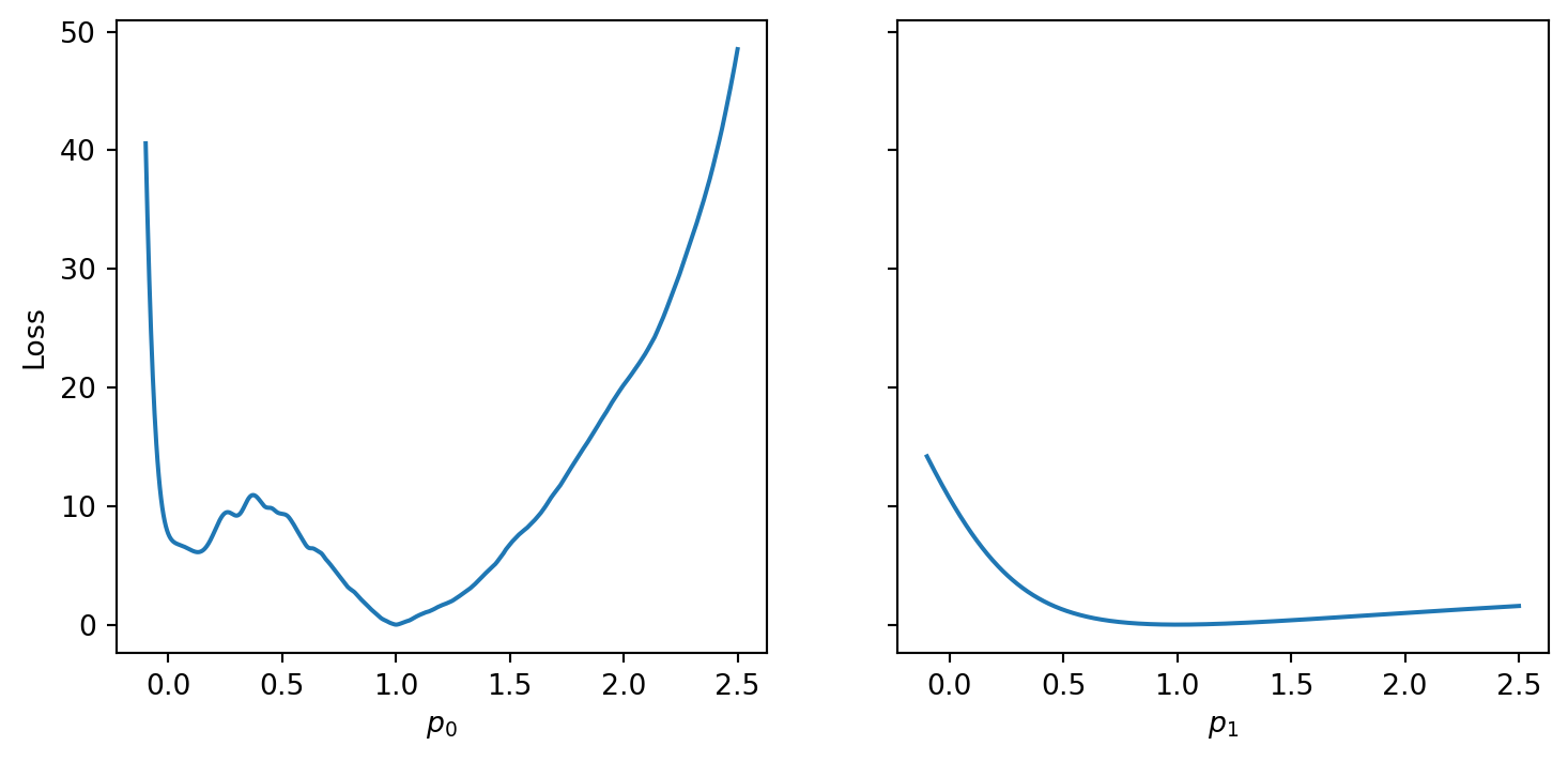
Although this behavior is somewhat typical of vanilla gradient descent, this model was pathologically chosen to be challenging. The curvature of the loss function for each parameter at the correct parameter values are as follows:
Plotting parameter loss curves
ps = np.linspace(-.1,2.5,1000)fig,axs = plt.subplots(1,2,sharey=True,figsize=(9,4))ax1,ax2 = axsax1.plot(ps,[loss(np.array([p_i,1])) for p_i in ps])ax1.set_xlabel("$p_0$"); ax1.set_ylabel("Loss")ax2.plot(ps,[loss(np.array([1,p_i])) for p_i in ps])ax2.set_xlabel("$p_1$")# plt.xlabel("$x$"); plt.ylabel("$y$"); plt.title("Model")plt.show()
In this loss, \(p_0\) demonstrates a plethora of local minima which could trap the descent algorithm while \(p_1\) has a small gradient which will slow down the convergence. The following methods are meant to simplify the choice of a learning rate while overcoming these specific convergence issues.
Adaptive steps
Due to the challenges of determining a good learning rate (especially in models with many parameters and large variance in loss gradients), many methods have been developed to automatically adjust the \(\alpha\) parameter with each step and for each parameter. One of the most common adaptive algorithms is called adagrad (for adaptive gradient. very creative). Originally developed to provide parameter specific learning rates in sparse problems (in the case that some parameters are only occasionally important) it scales the learning rate by a squared sum of previous gradients:
def adagrad(f_p,x0,alpha=.2,tol=1e-12,steps=1000): x = x0 xs = [x]# --------- NEW ----------- sum_sq_grad =0for s inrange(steps): sum_sq_grad = f_p(x)**2+ sum_sq_grad v_i =-alpha*f_p(x)/np.sqrt(sum_sq_grad)# ------------------------- xnew = x + v_iif np.linalg.norm(f_p(xnew)) < tol:print("Converged to objective loss gradient below {} in {} steps.".format(tol,s))return x,xselif np.linalg.norm(xnew - x) < tol:print("Converged to steady state of tolerance {} in {} steps.".format(tol,s))return x,xs x = xnew xs.append(x)print("Did not converge after {} steps (tolerance {}).".format(steps,tol))return x,xs
However, depending on the problem, this scaled learning rate may slow down convergence considerably. As an adjustment to remove this monotone decreasing learning rate, RMSprop attempts to balance the current gradient with a dampened version of the sum of squares of previous gradients from adagrad:
def rmsprop(f_p,x0,gamma=0.9,alpha=0.001,tol=1e-12,steps=1000): x = x0 xs = [x]# --------- NEW ----------- sum_sq_grad =0for s inrange(steps): sum_sq_grad = (1-gamma)*(f_p(x)**2) + gamma*sum_sq_grad v_i =-alpha*f_p(x)/np.sqrt(sum_sq_grad)# ------------------------- xnew = x + v_iif np.linalg.norm(f_p(xnew)) < tol:print("Converged to objective loss gradient below {} in {} steps.".format(tol,s))return x,xselif np.linalg.norm(xnew - x) < tol:print("Converged to steady state of tolerance {} in {} steps.".format(tol,s))return x,xs x = xnew xs.append(x)print("Did not converge after {} steps (tolerance {}).".format(steps,tol))return x,xs
This helps with the challenge of a monotone decreasing learning rate, but it introduces a dampening parameter \(\gamma\) that must be chosen (recommended values are \(\alpha = 0.001\) and \(\gamma = 0.9\)).
With momentum
Though the previous adaptive methods address the challenge of determining a learning rate, these methods are still likely to terminate in local minima. To address this issue, there are several methods which utilize a concept of “momentum” to propel iterations out of local minima with the hope of landing in the global minimum. This momentum is most simply added by incorporating previous gradients into the current update:
def gradient_descent_momentum(f_p,x0,gamma,alpha=0.01,tol=1e-12,steps=1000): x = x0 xs = [x]# --------- NEW ----------- sum_grad =0for s inrange(steps): sum_grad = f_p(x) + gamma*sum_grad v_i =-alpha*sum_grad# ------------------------- xnew = x + v_iif np.linalg.norm(f_p(xnew)) < tol:print("Converged to objective loss gradient below {} in {} steps.".format(tol,s))return x,xselif np.linalg.norm(xnew - x) < tol:print("Converged to steady state of tolerance {} in {} steps.".format(tol,s))return x,xs x = xnew xs.append(x)print("Did not converge after {} steps (tolerance {}).".format(steps,tol))return x,xs
where \(\gamma\) is a momentum parameter that determines how much of previous updates are kept for the current step (\(0 <= \gamma <=1\) where \(\gamma = 0\) includes no momentum).
However, iterations that include this momentum may jump right out of global minima and/or delay convergence. To incorporate a counterbalance to the momentum based on current success (to slow down in the right places), Nesterov acceleration adjusts the gradient according to an approximated step (to see how successful it may be in the future). By so doing, it can effectively reduce or increase the momentum according to the next future iteration:
def gradient_descent_nesterov(f_p,x0,gamma,alpha=0.01,tol=1e-12,steps=1000): x = x0 xs = [x]# --------- NEW ----------- sum_grad =0for s inrange(steps): sum_grad = f_p(x-gamma*v_i) + gamma*sum_grad v_i =-alpha*sum_grad# ------------------------- xnew = x + v_iif np.linalg.norm(f_p(xnew)) < tol:print("Converged to objective loss gradient below {} in {} steps.".format(tol,s))return x,xselif np.linalg.norm(xnew - x) < tol:print("Converged to steady state of tolerance {} in {} steps.".format(tol,s))return x,xs x = xnew xs.append(x)print("Did not converge after {} steps (tolerance {}).".format(steps,tol))return x,xs
where again \(\gamma\) is a momentum parameter. Notice that the only adjustment compared to vanilla gradient descent with momentum is calculating the gradient at an approximation of the next parameter values rather than at the current parameters.
Combining ideas
Of course, the ideas of adaptive gradients and momentum both address important issues and are not mutually exclusive, so they can both be used simultaneously (with the downside of adding more parameters to tune). Note that the adaptive step size methods (adagrad,RMSprop) use a sum of squares of the previous gradient while the momentum methods (gradient descent with momentum or Nesterov acceleration) use a sum of the previous gradient. These can be seen as the second moment and first moment of the previous gradients respectively. The Adam (adaptive moment estimation) method uses both of these gradient moments to incorporate both momentum and adaptivity:
Parameters \(\beta_1,\beta_2\) represent decay rates in incorporating previous moments into the update step.
Although this list is not comprehensive, it demonstrates the reasoning behind the common solutions for the challenges of using gradient descent in learning methods. For a more comprehensive list of recently proposed methods, see [5].
Automatic differentiation
Gradient descent methods rely on computing the gradient of the loss \(\nabla_p \mathcal{L}\) for a given parameter set \(\vec{p}^i\). For simple models, the gradients can be calculated by hand. However, for models with many nested functions and parameters (neural networks in particular) or methods whose form depends on hyperparameters, we will need an automated method. The “automatic differentiation” method is the solution to these challenges. Though it was developed for neural networks and mainly used there, its breadth of applications is only just becoming apparent. (Consider the Julia language which has worked hard to make automatic differentiation possible everywhere).
There are both “forward” and “backward” automatic differentiation methods, but we will consider only the forward which best demonstrates the “automatic” moniker. To do so, consider the first order expansion of two functions at a given point \(a\): \[
\begin{align*}
f(a + \epsilon) &= f(a) + \epsilon f'(a) \\
g(a + \epsilon) &= g(a) + \epsilon g'(a)
\end{align*}
\] where \(\epsilon\) is a small perturbation. Basic operations with these functions at this point can then be written as: \[
\begin{align*}
f + g &= [f(a) + g(a)] + \epsilon[f'(a) + g'(a)] \\
f - g &= [f(a) - g(a)] + \epsilon[f'(a) - g'(a)] \\
f \cdot g &= [f(a) \cdot g(a)] + \epsilon[f(a)\cdot g'(a) + g(a)\cdot f'(a)] \\
f \div g &= [f(a) \div g(a)] + \epsilon\left[\frac{f'(a)\cdot g(a) + f(a)\cdot g'(a)}{g(a)^2}\right]
\end{align*}
\] The derivatives are then represented by the \(\epsilon\) terms in the above equalities.
To implement this on a computer, you can create a new “Dual” number that performs additions, subtractions, multiplications, and divisions with the above operating rules (and can be extended for other functions: \(\sin,\cos,\exp\),etc).
Note
This is cumbersome and slow to implement in Python which is why large and complicated libraries have been written in C (tensorflow,pytorch,jax, and others).
It can be cleanly and easily implemented in Julia. To see a demonstration of this, see [6].
A quick demonstration of a simple implementation of this is as follows [7]. Define a dual number class:
class DualNumber:def__init__(self, val, der):self.val = valself.der = derdef__add__(self, other):ifisinstance(other, DualNumber):# DualNumber + DualNumberreturn DualNumber(self.val + other.val, self.der + other.der)else:# DualNumber + a numberreturn DualNumber(self.val + other, self.der)def__radd__(self, other):# a number + DualNumberreturnself.__add__(other)def__mul__(self,other):ifisinstance(other, DualNumber):# DualNumber * DualNumberreturn DualNumber(self.val * other.val, self.val*other.der +self.der*other.val)else:# DualNumber * a numberreturn DualNumber(self.val * other, self.der * other)def__rmul__(self,other):# a number * DualNumberreturnself.__mul__(other)def__pow__(self,power):# DualNumber ^ a numberreturn DualNumber(self.val ** power, self.der * power * (self.val ** (power -1)))def__repr__(self):# Printing a DualNumberreturn"DualNumber({},{})".format(self.val,self.der)dual1 = DualNumber(1,2); dual2 = DualNumber(3,4); other =5print(dual1,"+",dual2,"=",dual1+dual2)print(dual1,"+",other,"=",dual1+other)print(dual1,"*",dual2,"=",dual1*dual2)print(dual1,"*",other,"=",dual1*other)print(dual1,"^",2,"=",dual1**2)
This seems simple, but by using a few rules like this, we can compute simple polynomial derivatives at a point automatically. For example, computing the derivative of \(f(x) = 3x^3 + 2x + 4\) at \(x=2\). We first initialize the function and the dual number \((2,1)\) (\(1\) because the derivative of \(x\) is \(1\)).
We then pass the dual number through the polynomial function, unpack the results, and compare the result with the true derivative \(f'(2)\):
poly_dual = f(dualx)dual_val = poly_dual.val; dual_der = poly_dual.dertrue_der = df(x)print("True derivative at x=2: ", true_der)print("Dual number derivative: ", dual_der)
True derivative at x=2:  38
Dual number derivative:  38
Using the rules for dual numbers we provided above, the derivative “automatically” popped out of the polynomial evaluation.
In contrast with the forward method, the backward method keeps a log of the operations performed and then uses defined chain rules (similar to how we defined rules for the forward pass) to backtrack from the final output back to the start. This approach is more efficient when the dimension of the gradient is large and that of the output small. Forward evaluation is more efficient when the dimension of the gradient is small and that of the output large.
All in all, automatic differentiation is programming with hard-coded differential rules for primitive operations. It can also require keeping track of which operations happen and in what order. Implementing such a method relies heavily on computer science techniques since it boils down to parsing operation calls. This represents one of the clearest differences in the approaches of machine learning to those of statistics or optimization due to its computer language-heavy principles. Through this lens, machine learning could be viewed as “inferential statistics using new tools from computer science for non-traditional problems.”
Further Exploration
Each of the parameters for the gradient descent methods was chosen by hand for the above animations. Try adjusting the starting point and parameters for each to get a feel for how they behave.
Try splitting the sample data into a training and a testing set. Use the training set and one of the gradient descent methods to fit some parameters, then see how well the model generalizes to the testing set with those parameters.
Try implementing another gradient descent method from [4] using the given methods as a template.
Add the missing subtraction (__sub__, __rsub__) and division (__truediv__, __rtruediv__) methods in the DualNumber class and play around with automatically differentiation functions using those operators (you can use this as a reference). You can also make functions such as sin,cos, or exp that are meant to compute with DualNumbers.
numpy - Creating, manipulating, and operating (linear algebra, fft, etc.) on multi-dimensional arrays. A list of packages built on numpy for a variety of domains can be found on the homepage under the ECOSYSTEM heading.
scipy - Fundamentals in optimization, integration, interpolation, differential equations, statistics, signal processing, etc.
matplotlib - Static or interactive plots and animations
scikit-learn - Standard machine learning tools and algorithms built on numpy, scipy, and matplotlib
pandas - Easily represent, manipulate, and visualize structured datasets (matrices with names for columns and rows)
keras - High level neural network framework built on tensorflow
tensorflow - In depth neural network framework focused on ease and production
pytorch - In depth neural network framework focused on facilitating the path from research to production
scikit-image - Image processing algorithms and tools
Julia is a fairly new language that has been mainly proposed as an alternative to Python and Matlab, though it is general use. Its strength and its weakness is that it is “just-in-time” compiled (meaning your code is automatically analyzed and compiled just before it is run). A clever language design combined with just-in-time compilation makes Julia as clear to read and write as Python while being much faster. It can even approach the speed of C when written carefully. However, the just-in-time compilation and type system remove a chunk of the interactive convenience of Python and its young age also means that it does not have the volume of packages that Python does.
Nonetheless, it is an elegant and high-performance language to use and has shown rapid growth recently. Concise, simple, and easy to read and contribute to packages have been quickly emerging and it already provides many useful tools. As a result, it is worth describing it’s installation process, environment management, and noteable packages.
Installation
The officially supported method of installation for Julia is now using the juliaup version manager. The installer can be downloaded from the Windows store on Windows or run on MacOS or Linux with:
curl-fsSL https://install.julialang.org |sh
Environments
Julia comes with a standard environment and package manager named Pkg. Interestingly, the easiest way to use it is to run the Julia REPL (read-eval-print-loop), i.e. to run julia interactively. You can do so by typing julia into the terminal. You will then be presented with a terminal interface such as:
Type ? and hit enter to get options in this mode. We can create and activate a new environment called workshop with the command:
(@v1.8) pkg> activate --shared workshop
Note that the --shared flag will make a “global” environment that can be accessed from any directory. If we were to leave out this flag, Pkg would put a Project.toml and Manifest.toml file in the current directory that contain the name of the environment, its installed packages, and their dependencies. This can be useful to easily isolate and share environments. After running this command, our Pkg mode will have changed to represent the active environment:
(@workshop) pkg>
Installing packages
To install some packages in the active environment, write:
These packages will install and precompile. To test one of them, press backspace to leave Pkg mode and input:
julia> using Plots[ Info: Precompiling Plots [91a5bcdd-55d7-5caf-9e0b-520d859cae80]julia> x = range(0,10,100);julia> y = sin.(x);julia> plot(x,y)
This should show a plot of a simple \(\sin\) curve. Note that the precompilation of Plots took some time. However, this will not need to occur again until the package is updated. Also note that the call to plot(x,y) took some time. This is due to the just-in-time compilation. Now that the compilation has been done for inputs of the types of x and y, if you run plot(x,y) again, it should be almost instantaneous.
Cleaning up
To deactivate the environment, enter the Pkg mode again by pressing ] on an empty line, then enter:
(@workshop) pkg> activate
To delete the environment we created you can delete the environment folder at the listed location at creation. This is usually /home/user/.julia/environments/workshop on MacOS or Linux.
As compared to Python, Julia has many scientific computing tools built into its standard library. Thus, a lot of the functionality found in numpy are loaded by default. On the other hand, because of the interoperability of the language and the reduced need for a polyglot codebase (i.e. needing C and Fortran code for a Python package to be fast), packages are usually much smaller modules in Julia. For example, the functionality of the scipy package in Python can be found spread across possibly a dozen different packages in Julia. This is convenient to only load and use what you need, but inconvenient in that it may require more searching to find and the interfaces may not be standardized. The following are some packages that roughly recreate the essential Python packages here.
jupyter - Pluto.jl although you can use Julia with Jupyter via IJulia.jl
References
[1]
K. P. Murphy, Machine Learning: A Probabilistic Perspective (MIT press, 2012).
[2]
G. James, D. Witten, T. Hastie, and R. Tibshirani, An Introduction to Statistical Learning, Vol. 112 (Springer, 2013).
[3]
T. Hastie, R. Tibshirani, J. H. Friedman, and J. H. Friedman, The Elements of Statistical Learning: Data Mining, Inference, and Prediction, Vol. 2 (Springer, 2009).

 However, depending on the problem, this scaled learning rate may slow down convergence considerably. As an adjustment to remove this monotone decreasing learning rate,
  This helps with the challenge of a monotone decreasing learning rate, but it introduces a dampening parameter
  where
where  where again
  Parameters