Workshop 3: Data-driven discovery via Sparse Identification of Nonlinear Dynamics (SINDy) with neural network approximation and differentiation

Author

Connor Robertson

Overview

One common hallmark of popular machine learning methods is their “black-box” nature. Since many of these methods are meant solely for prediction, this has not been too much of an issue. After all, a black box method can be as complex as needed since it does not need to be analyzed after the fact. This mentality has given birth to increasingly complex but effective models (just take a look at the model that defeated the worlds best Go player).

However, there has been some recent interest in models that can be understood and analyzed. This is particularly true in the scientific realm, where practicioners looking to use machine learning would like to get an idea of the mechanisms underlying their system of study. In order to do so, new tools have been created and old, interpretable tools, such as linear regression, have been adapted to meet this challenge.

Many of these new, interpretable, models have been named “data-driven model discovery.” Their goals is to model collected data from a system with machine learning tools to determine a human-readable model.

Sparse Identification of Nonlinear Dynamics

One method for model discovery as described above is called Sparse Identification of Nonlinear Dynamics (SINDy) [1]. The goal of this method is to extract the most probable differential equation directly from data of the important state variables of a continuum system.

Setting up linear problem

As its name suggests, this method works discover models for linear or nonlinear systems. It is based on a simple idea that nonlinear differential equations can be expressed as a linear combination of nonlinear terms [2]. Assuming we are looking at the nonlinear time evolution of some quantity, this could then be written as the sum of \(K\) nonlinear terms: \[ u_t(x,t) = \xi_1\mathcal{N}_1(u,x,t) + \ldots + \xi_K\mathcal{N}_K(u,x,t) \] If we can then determine what nonlinear terms are possible \(\mathcal{N}_i(u,x,t)\), we can sift through these terms to determine which best contribute to the time evolution of the system.

Ultimately, this boils down to a regression problem. Given some space and time samples of our state variable: \(u(x_i,t_j)\) for \(i \leq N\) and \(j \leq M\), we can consider the linear system: \[ u_t(x_i,t_j) = \xi_1\mathcal{N}_1(u_{ij},x_i,t_j) + \ldots + \xi_K\mathcal{N}_K(u_{ij},x_i,t_j) \] Expanded for all the data samples (flattened across space and time), this can be written as the system: \[ \begin{bmatrix} u_t(x_1, t_1) \\ \vdots \\ u_t(x_N, t_1) \\ \vdots \\ u_t(x_N, t_M) \\ \end{bmatrix} = \begin{bmatrix} \mathcal{N}_1(x_1, t_1) & \ldots & \mathcal{N}_K(x_1, t_1) \\ \vdots & & \vdots \\ \mathcal{N}_1(x_N, t_1) & \ldots & \mathcal{N}_K(x_1, t_1) \\ \vdots & & \vdots \\ \mathcal{N}_1(x_N, t_M) & \ldots & \mathcal{N}_K(x_1, t_1) \end{bmatrix} \vec{\xi} \tag{1}\]

Solving this system is then a straightforward linear regression.

Determining nonlinear “library” of terms

Determining what \(\mathcal{N}_i(u,x,t)\) are reasonable for the system is somewhat of a traditional modeling problem. Are there any symmetries in the system that need to be satisfied? Is there periodic behavior that might warrant inclusion of trignometric terms? What order of polynomial interactions are possible for the system?

The most common library of terms for a 1D function is to put together polynomial interactions with spatial derivatives. Such a library up to 3rd order polynomials and derivatives could be written: \[ \begin{align*} \mathcal{N}_1(u,x,t) &= u\\ \mathcal{N}_2(u,x,t) &= u^2\\ &\vdots \\ \mathcal{N}_i(u,x,t) &= u_x\\ \mathcal{N}_{i+1}(u,x,t) &= u_x^2\\ &\vdots \\ \mathcal{N}_K(u,x,t) &= u^3u_{xxx}\\ \end{align*} \]

Numerical differentiation of the terms

In order to actually compute the values in the linear system written in Equation 1, we must compute numerical derivatives in both \(t\) and in \(x\). This isn’t an issue if we have smooth, reliable data and can be quickly computed with finite differences.

However, the intent of this method is to use data samples \(u(x_i,t_j)\) that are collected from the real world, implying that they will each be polluted with some level of noise. There have been several classical methods presented for dealing with numerical differentiation of noisy data that could be used, but generally the methods revolve around an approximate fitting of a differentiable function basis to the data. Notable among these are:

  • Local polynomial regression (LOESS [3], Savitsky-Golay filter [4], etc.)
  • Radial basis functions (Gaussian kernel)
  • Smoothing splines
  • Least squares spectral analysis (LSSA)

These can be written along the lines of: \[ \underset{\vec{c}}{\text{argmin}} \; \sum_{i,j}^{N,M}\|u(x_i,t_j) - F(x_i,t_j,\vec{c})\|_2 \] where \[ F(x_i,t_j,\vec{c}) = \sum_l^L c_l \phi_l(x_i,t_j) \] and \(\phi\) represents our chosen basis function. Once computed, we can easily approximate derivatives of \(u\) via: \[ u_x(x_i,t_j) \approx F_x(x_i,t_j,\vec{c}) = \sum_l^L c_l \frac{d}{dx}\phi_l(x_i,t_j) \]

Each of these has the goal of smoothing the given data while simultaneously providing an exact derivative of the approximation. This is a similar idea as we have discussed with automatic differentiation of neural networks. In fact, you could consider fitting a neural network to be the same as fitting a randomly initialized nested basis of nonlinear functions (since they are dense according to the universal approximation theorem). We will explore this idea in the example problem in Section 3.

Sparse regression

Once the matrix in Equation 1 has been created using numerical differentiation, it remains to sift through the nonlinear terms to determine which, if any, contribute to the time evolution of our state variable of interest. It is usually reasonable to consider that not all the nonlinear terms should be included in the equation, so we would like to determine the most parsimonious (smallest) combination of them that will capture our desired qualitative and quantitative behavior in the system.

There are two main families of sparse regression methods:

Greedy methods: Iterative add/remove terms that best match the time derivative in some metric (\(R^2\) coefficient of determination, Akaike Information Criteria (AIC), etc.).

  • Forward selection: Start with no terms, add one by one according to which maximizes \(R^2\) or AIC at each step
  • Backward selection: Start with all terms, remove one by one according to which least reduces \(R^2\) or AIC
  • (Orthogonal) Matching pursuit: Start with no terms, add one by one according to which maximizes correlation (orthogonalizing after each step)

Regularization methods: Add a penalty to the regression for having too many terms or large coefficients \(\xi_i\). These can be written roughly as: \[ \underset{\vec{\xi}}{\text{argmin}}\; \|u_t(x_i,t_j) - \mathbf{\mathcal{N}}(u_{ij},x_i,t_j) \cdot \vec{\xi}\|_2^2 + \lambda \|\xi\|_C \]

  • Ridge regression: Let \(C=2\) forcing coefficients \(\vec{\xi}\) to be smaller. We hope that important coefficients will remain larger while unimportant ones shrink.
  • Lasso regression: Let \(C=1\) forcing coefficients \(\vec{\xi}\) to be smaller and various to be set to 0 (due to the geometry of the 1-norm).
  • 0-norm regression: Let \(C=0\) which is a measure that counts the number of nonzero coefficients in \(\vec{\xi}\). Computing this usually requires a combination of regularization and relaxation best captured by the SR3 method [5].

Combinations of these two methods which iterative perform regularization methods removing terms with small coefficients according to a given threshold have also been proposed (Sequential Threshold Ridge Regression [6] or the original SINDy algorithm [1]).

Summary of the method

In summary, the procedure to use SINDy is as follows:

  1. Collect sample points of a continuum state variable of interest \(u(x_i,t_j)\)
  2. Form a “library” of possible terms for the differential model of the system \(\mathcal{N}_k(u,x,t)\)
  3. Compute the libary at sample points using noise robust numerical differentiation to compute both \(u_t(x_i,t_j)\) and \(\mathcal{N}_k(u_{ij},x_i,t_j)\)
  4. Use sparse regression to determine a sparse vector \(\vec{\xi}\) which closely approximates \(u_t(x_i,t_j) = \xi_1\mathcal{N}_1(u_{ij},x_i,t_j) + \ldots + \xi_K\mathcal{N}_K(u_{ij},x_i,t_j)\)

To really explore this method, we will walk through this process using simulated traveling wave data in Section 3 and using real extracted data in Section 5.

Application to simulated wave data

Note

For this workshop you will need to install the following packages:

mamba install numpy matplotlib py-pde sympy jax optax flax scikit-learn scikit-image av

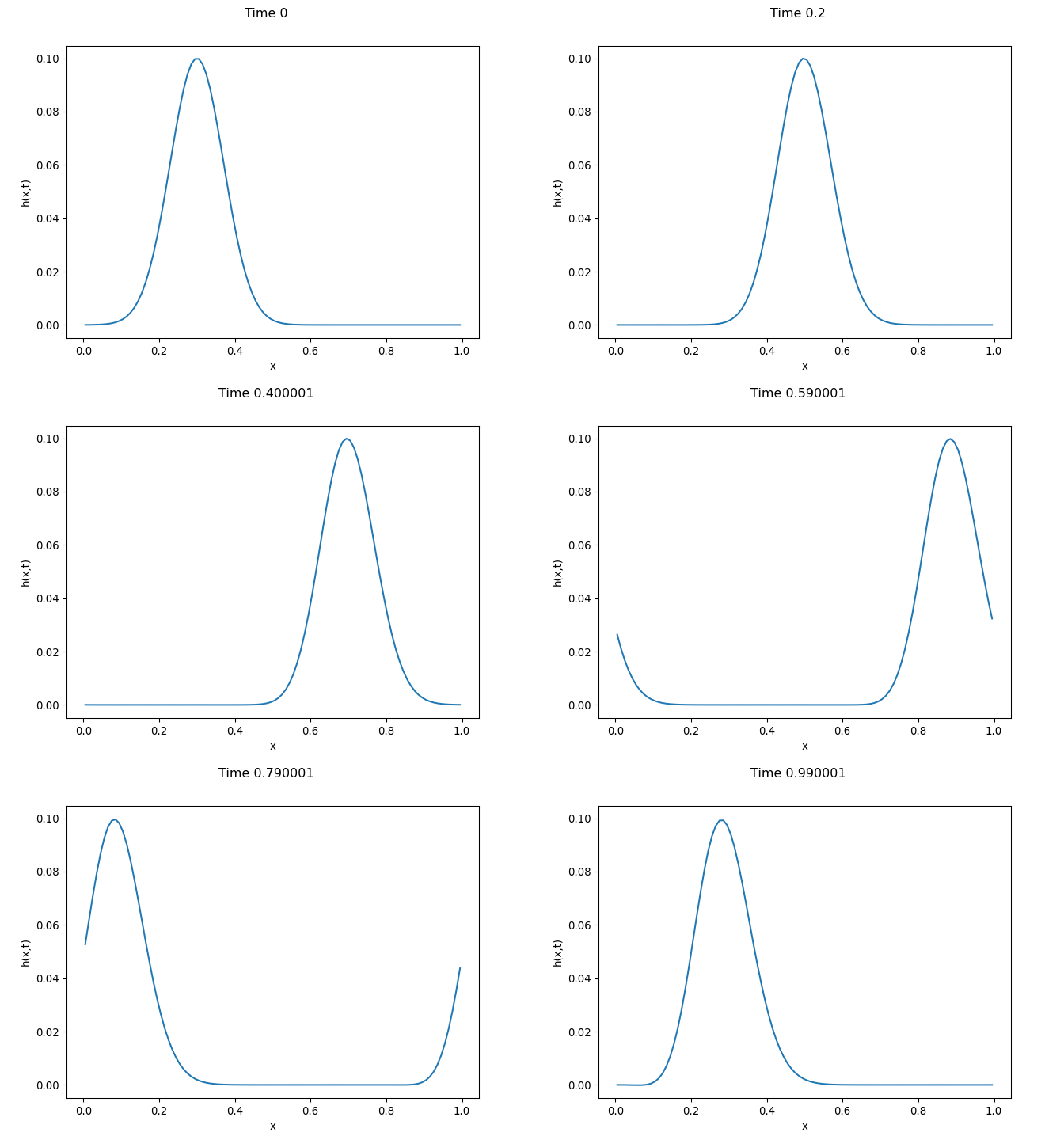
Given some data generated via finite differences of the simple advection equation: \[ h_t(x,t) = h_x(x,t) \] with periodic boundaries and a Gaussian initial condition, we have the following measurement of state variable \(h\) (height of the wave):

Generate simple wave data
import numpy as np
import pde
import matplotlib.pyplot as plt

# Domain
xmax = 1.0
nx = 100
dt = 1e-6
tmax = 1.0-2*dt
save_dt = 0.01
init_cond = ".1*exp(-(1/.01)*(x-0.3)**2)"

grid = pde.CartesianGrid([(0.0,xmax)],nx,periodic=True)
h = pde.ScalarField.from_expression(grid,init_cond,label="h(x,t)")
eq = pde.PDE({"h": "-d_dx(h)"})
storage = pde.MemoryStorage()

result = eq.solve(h,t_range=tmax,dt=dt,tracker=storage.tracker(save_dt),ret_info=False)

# pde.plot_kymograph(storage)
movie = pde.visualization.movie(storage,"simple_wave.gif")

h=np.array(storage.data)
x=storage.grid.coordinate_arrays[0]
t=np.array(storage.times)
np.savez("simple_wave.npz",h=h,x=x,t=t)
plt.close()

Generating nonlinear library

Generating a library can be most easily accomplished using the sympy symbolic math Python library. To be overly thorough, we will generate up to 4th order polynomial combinations of up to 4th order spatial derivatives.

We can first initialize our spatial and state variables:

import sympy as sp

x_sym,t_sym = sp.symbols("x t")
h_sym = sp.Function("h")

Given a specified order, we can now create symbolic derivative terms (constructed to be most legible):

# Library parameters
max_poly_order = 4
max_diff_order = 4

diff_terms = [h_sym(x_sym,t_sym)]
diff_terms += [sp.Function(str(h_sym)+"_"+(i*str(x_sym)))(x_sym,t_sym) for i in range(1,max_diff_order+1)]
print(diff_terms)
[h(x, t), h_x(x, t), h_xx(x, t), h_xxx(x, t), h_xxxx(x, t)]

Now, combining these into polynomials up to 4th order (again, this is overkill, but for a system you don’t fully understand, you may want to have a very complete library):

from itertools import combinations_with_replacement

terms = []
for po in range(max_poly_order+1):
    if po == 0:
        term = sp.core.numbers.One()
    else:
        combos = combinations_with_replacement(diff_terms,po)
        for combo in combos:
            term = 1
            for combo_term in combo:
                term *= combo_term
            terms.append(term)
print(terms)
[h(x, t), h_x(x, t), h_xx(x, t), h_xxx(x, t), h_xxxx(x, t), h(x, t)**2, h(x, t)*h_x(x, t), h(x, t)*h_xx(x, t), h(x, t)*h_xxx(x, t), h(x, t)*h_xxxx(x, t), h_x(x, t)**2, h_x(x, t)*h_xx(x, t), h_x(x, t)*h_xxx(x, t), h_x(x, t)*h_xxxx(x, t), h_xx(x, t)**2, h_xx(x, t)*h_xxx(x, t), h_xx(x, t)*h_xxxx(x, t), h_xxx(x, t)**2, h_xxx(x, t)*h_xxxx(x, t), h_xxxx(x, t)**2, h(x, t)**3, h(x, t)**2*h_x(x, t), h(x, t)**2*h_xx(x, t), h(x, t)**2*h_xxx(x, t), h(x, t)**2*h_xxxx(x, t), h(x, t)*h_x(x, t)**2, h(x, t)*h_x(x, t)*h_xx(x, t), h(x, t)*h_x(x, t)*h_xxx(x, t), h(x, t)*h_x(x, t)*h_xxxx(x, t), h(x, t)*h_xx(x, t)**2, h(x, t)*h_xx(x, t)*h_xxx(x, t), h(x, t)*h_xx(x, t)*h_xxxx(x, t), h(x, t)*h_xxx(x, t)**2, h(x, t)*h_xxx(x, t)*h_xxxx(x, t), h(x, t)*h_xxxx(x, t)**2, h_x(x, t)**3, h_x(x, t)**2*h_xx(x, t), h_x(x, t)**2*h_xxx(x, t), h_x(x, t)**2*h_xxxx(x, t), h_x(x, t)*h_xx(x, t)**2, h_x(x, t)*h_xx(x, t)*h_xxx(x, t), h_x(x, t)*h_xx(x, t)*h_xxxx(x, t), h_x(x, t)*h_xxx(x, t)**2, h_x(x, t)*h_xxx(x, t)*h_xxxx(x, t), h_x(x, t)*h_xxxx(x, t)**2, h_xx(x, t)**3, h_xx(x, t)**2*h_xxx(x, t), h_xx(x, t)**2*h_xxxx(x, t), h_xx(x, t)*h_xxx(x, t)**2, h_xx(x, t)*h_xxx(x, t)*h_xxxx(x, t), h_xx(x, t)*h_xxxx(x, t)**2, h_xxx(x, t)**3, h_xxx(x, t)**2*h_xxxx(x, t), h_xxx(x, t)*h_xxxx(x, t)**2, h_xxxx(x, t)**3, h(x, t)**4, h(x, t)**3*h_x(x, t), h(x, t)**3*h_xx(x, t), h(x, t)**3*h_xxx(x, t), h(x, t)**3*h_xxxx(x, t), h(x, t)**2*h_x(x, t)**2, h(x, t)**2*h_x(x, t)*h_xx(x, t), h(x, t)**2*h_x(x, t)*h_xxx(x, t), h(x, t)**2*h_x(x, t)*h_xxxx(x, t), h(x, t)**2*h_xx(x, t)**2, h(x, t)**2*h_xx(x, t)*h_xxx(x, t), h(x, t)**2*h_xx(x, t)*h_xxxx(x, t), h(x, t)**2*h_xxx(x, t)**2, h(x, t)**2*h_xxx(x, t)*h_xxxx(x, t), h(x, t)**2*h_xxxx(x, t)**2, h(x, t)*h_x(x, t)**3, h(x, t)*h_x(x, t)**2*h_xx(x, t), h(x, t)*h_x(x, t)**2*h_xxx(x, t), h(x, t)*h_x(x, t)**2*h_xxxx(x, t), h(x, t)*h_x(x, t)*h_xx(x, t)**2, h(x, t)*h_x(x, t)*h_xx(x, t)*h_xxx(x, t), h(x, t)*h_x(x, t)*h_xx(x, t)*h_xxxx(x, t), h(x, t)*h_x(x, t)*h_xxx(x, t)**2, h(x, t)*h_x(x, t)*h_xxx(x, t)*h_xxxx(x, t), h(x, t)*h_x(x, t)*h_xxxx(x, t)**2, h(x, t)*h_xx(x, t)**3, h(x, t)*h_xx(x, t)**2*h_xxx(x, t), h(x, t)*h_xx(x, t)**2*h_xxxx(x, t), h(x, t)*h_xx(x, t)*h_xxx(x, t)**2, h(x, t)*h_xx(x, t)*h_xxx(x, t)*h_xxxx(x, t), h(x, t)*h_xx(x, t)*h_xxxx(x, t)**2, h(x, t)*h_xxx(x, t)**3, h(x, t)*h_xxx(x, t)**2*h_xxxx(x, t), h(x, t)*h_xxx(x, t)*h_xxxx(x, t)**2, h(x, t)*h_xxxx(x, t)**3, h_x(x, t)**4, h_x(x, t)**3*h_xx(x, t), h_x(x, t)**3*h_xxx(x, t), h_x(x, t)**3*h_xxxx(x, t), h_x(x, t)**2*h_xx(x, t)**2, h_x(x, t)**2*h_xx(x, t)*h_xxx(x, t), h_x(x, t)**2*h_xx(x, t)*h_xxxx(x, t), h_x(x, t)**2*h_xxx(x, t)**2, h_x(x, t)**2*h_xxx(x, t)*h_xxxx(x, t), h_x(x, t)**2*h_xxxx(x, t)**2, h_x(x, t)*h_xx(x, t)**3, h_x(x, t)*h_xx(x, t)**2*h_xxx(x, t), h_x(x, t)*h_xx(x, t)**2*h_xxxx(x, t), h_x(x, t)*h_xx(x, t)*h_xxx(x, t)**2, h_x(x, t)*h_xx(x, t)*h_xxx(x, t)*h_xxxx(x, t), h_x(x, t)*h_xx(x, t)*h_xxxx(x, t)**2, h_x(x, t)*h_xxx(x, t)**3, h_x(x, t)*h_xxx(x, t)**2*h_xxxx(x, t), h_x(x, t)*h_xxx(x, t)*h_xxxx(x, t)**2, h_x(x, t)*h_xxxx(x, t)**3, h_xx(x, t)**4, h_xx(x, t)**3*h_xxx(x, t), h_xx(x, t)**3*h_xxxx(x, t), h_xx(x, t)**2*h_xxx(x, t)**2, h_xx(x, t)**2*h_xxx(x, t)*h_xxxx(x, t), h_xx(x, t)**2*h_xxxx(x, t)**2, h_xx(x, t)*h_xxx(x, t)**3, h_xx(x, t)*h_xxx(x, t)**2*h_xxxx(x, t), h_xx(x, t)*h_xxx(x, t)*h_xxxx(x, t)**2, h_xx(x, t)*h_xxxx(x, t)**3, h_xxx(x, t)**4, h_xxx(x, t)**3*h_xxxx(x, t), h_xxx(x, t)**2*h_xxxx(x, t)**2, h_xxx(x, t)*h_xxxx(x, t)**3, h_xxxx(x, t)**4]
Approximating data

In order to provide numerical derivatives of our data, we will use a neural network approximation.

Note

This is far beyond what is necessary for this particular setting, but is a method that can generalize to data not on a uniform grid and in high dimension, which can be useful. The lack of requirement for a grid can also help with robustly fitting to noisy data by using a train-test methodology in Section 4 which classical basis functions do not handle well. Using neural networks in this way as a combination with SINDy is explored more in [7].

To begin, we will be using the Google developed flax neural network framework which is built on their jax automatic differentiation library and the optax optimization library. The reason for this will become clearer when we consider taking a fourth order derivative in \(x\) of the network, a task which many other popular frameworks (pytorch, keras, tensorflow, etc.) cannot do (at least not nearly as concisely). However, the jax library is state-of-the-art for automatic differentiation and is used heavily for differentiable programming and neural network research today (see Appendix for more information).

Creating the neural network model

First, we will create a simple dense neural network model using the \(\tanh\) activation (to ensure a smooth approximation):

import flax.linen as nn

class MyNet(nn.Module):
    @nn.compact
    def __call__(self, x):
        x = nn.Dense(60)(x)
        x = nn.tanh(x)
        x = nn.Dense(12)(x)
        x = nn.tanh(x)
        x = nn.Dense(1)(x)
        return x

This model will take an input of \((x_i,t_j)\) (a dimension 2 array), linearly map it to a dimension 60 space, apply a tanh activation, linearly map to a dimension 12 space, apply a tanh activation, then linearly map to a dimension 1 output (this particular width and depth was chosen arbitrarily).

We next initialize the parameters of the network (each of the linear transformation matrices) and print out the dimensions of the corresponding arrays:

import jax
jax.config.update("jax_platform_name", "cpu")

# Random generator seed
rng1,rng2 = jax.random.split(jax.random.PRNGKey(42))
random_data = jax.random.normal(rng1,(2,))
model1 = MyNet()
params1 = model1.init(rng2,random_data)
print(jax.tree_util.tree_map(lambda x: x.shape, params1))
FrozenDict({
    params: {
        Dense_0: {
            bias: (60,),
            kernel: (2, 60),
        },
        Dense_1: {
            bias: (12,),
            kernel: (60, 12),
        },
        Dense_2: {
            bias: (1,),
            kernel: (12, 1),
        },
    },
})
Note

The confusing tree_util.tree_map command is a convenience function for mapping a function (in this case lambda x: x.shape) across a set of different objects. This is useful because these objects can be arrays, dictionaries, lists, classes (i.e. other neural networks), etc.

Loading and processing data

In order to fit this model to the data, we must load the data into batches of \((x_i,t_j,u(x_i,t_j))\) points. Since our data is known to be quite smooth and we want to maximize the fit, we will use batches of size 10000:

import jax.numpy as jnp

def load_data(data_path,noise_scale=0,norm=True):
    raw_data = np.load(data_path)
    h = raw_data["h"].astype(jnp.float32)
    x = raw_data["x"].astype(jnp.float32)
    t = raw_data["t"].astype(jnp.float32)

    # Add noise if needed
    h += noise_scale*jnp.std(h)*np.random.normal(size=h.shape)

    # Mean center, std center data
    if norm:
        h = (h - jnp.mean(h)) / jnp.std(h)
        x = (x - jnp.mean(x)) / jnp.std(x)
        t = (t - jnp.mean(t)) / jnp.std(t)
    return x,t,h

def batch_data(x,t,h,batch_size):
    # Split data into batches
    data = []
    for i in range(0,len(x),batch_size):
        temp_xt = jnp.vstack((x[i:i+batch_size], t[i:i+batch_size])).T
        temp_h = h[i:i+batch_size].reshape((-1,1))
        data.append((temp_xt,temp_h))
    return data

x,t,h = load_data("simple_wave.npz")
X,T = jnp.meshgrid(x,t)
data = batch_data(X.flatten(),T.flatten(),h.flatten(),10000)

Note that the data needed to be centered and scaled to have a mean of \(\bar{h}=0\) and standard deviation of \(\overline{(h - \bar{h})}=1\) in order to best use the \(\tanh\) activation (which extends from -1 to 1).

Training the model

We will use the mean squared error fit of the data to our neural network output (just in time compiled with @jax.jit for maximum speed):

@jax.jit
def mse(params,input,targets):
    def squared_error(x,y):
        pred = model1.apply(params,x)
        return jnp.mean((y - pred)**2)
    return jnp.mean(jax.vmap(squared_error)(input,targets),axis=0)
loss_grad_fn = jax.value_and_grad(mse)

With this loss defined, we initialize an ADAM optimizer and optimizer state and wrap the loss function to return both the output and gradient:

import optax

learning_rate = 1e-2
tx = optax.adam(learning_rate)
opt_state = tx.init(params1)

We can now train the model to take in \((x_i,t_j)\) and output \(u(x_i,t_j)\). Performing 1000 iterations over the data, we will print the mean squared error on the data as we proceed with the training:

epochs = 1000
all_xt = jnp.array([data[i][0] for i in range(len(data))])
all_h = jnp.array([data[i][1] for i in range(len(data))])
for i in range(epochs):
    xt_batch = data[i%len(data)][0]
    h_batch = data[i%len(data)][1]
    loss_val, grads = loss_grad_fn(params1, xt_batch, h_batch)
    updates, opt_state = tx.update(grads, opt_state)
    params1 = optax.apply_updates(params1, updates)
    if i % 100 == 0:
        train_loss = mse(params1,all_xt,all_h)
        print("Training loss step {}: {}".format(i,train_loss))
Training loss step 0: 1.089915156364441
Training loss step 100: 0.16426406800746918
Training loss step 200: 0.09340785443782806
Training loss step 300: 0.01907801441848278
Training loss step 400: 0.0014767495449632406
Training loss step 500: 0.000554197293240577
Training loss step 600: 0.00032399679184891284
Training loss step 700: 0.00021209089027252048
Training loss step 800: 0.0001550953311379999
Training loss step 900: 0.0001249150518560782

As you can tell, this procedure is somewhat more manual than other libraries such as keras but keep you closer to the details, allowing for more flexibility in implementation.

Validating fit

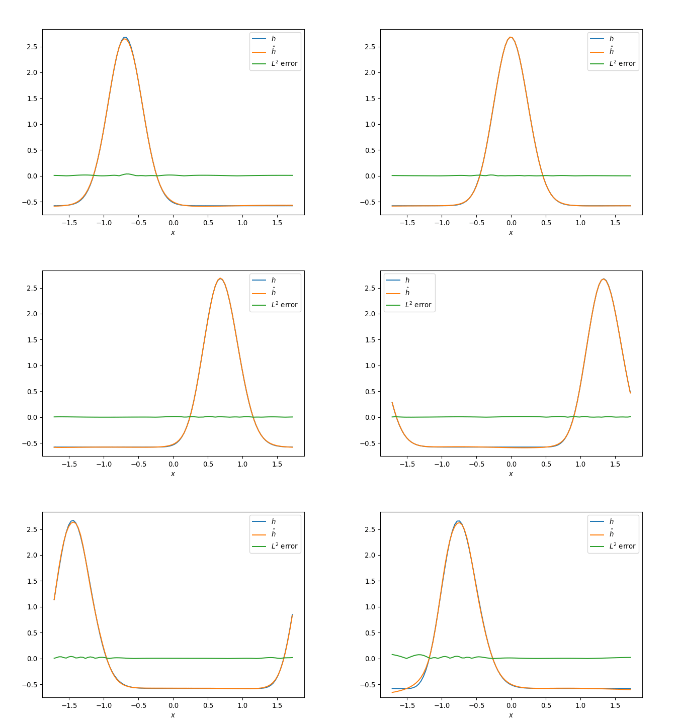
The fit to the model can be visualized as follows:

import matplotlib.animation as anim

X,T = jnp.meshgrid(x,t)
xt_points = jnp.vstack([X.flatten(),T.flatten()]).T
hhat1 = model1.apply(params1,xt_points).reshape(X.shape)
diff = np.sqrt((h - hhat1)**2)

def animate_data(x,t,data_list,labels):
    fig = plt.figure()
    plt.xlabel("$x$")
    plots = []

    for i in range(len(data_list)):
        plot = plt.plot(x,data_list[i][0,:],label=labels[i])[0]
        plots.append(plot)

    def anim_func(j):
        for i in range(len(plots)):
            plots[i].set_ydata(data_list[i][j,:])
        return plots

    plt.legend()
    approx_anim = anim.FuncAnimation(fig, anim_func, range(len(t)))
    return approx_anim

animation1 = animate_data(x,t,[h,hhat1,diff],["$h$","$\hat{h}$","$L^2$ error"])
animation1.save("clean_h_compare.gif")
plt.close()

Numerically differentiating the neural network model

The original reason to fit this model to the data was to be able to construct each of the terms in our nonlinear libary for the system. In order to differentiate the model, we must wrap it in a function that takes our inputs and returns the output.

def model_for_diff(x,t):
    new_x = jnp.array([x,t])
    return model1.apply(params1, new_x)[0]

# Take a derivative with respect to the first input (x) at point (x_i,t_j)
x_i = 0.3; t_j = 0.3
jax.grad(model_for_diff,0)(x_i,t_j)
Array(0.02786821, dtype=float32, weak_type=True)
Note

If we were to differentiate the model directly, we would compute derivatives for all the parameters! This is the main challenge with using other neural network frameworks for this kind of function approximation.

Applying this iteratively, we can construct derivatives \(h_x(x,t), \ldots, h_{xxxx}(x,t)\) as is required by our library:

diff_term_values = {}
for i in range(max_diff_order+1):
    diff_func = model_for_diff
    # Iteratively apply derivatives
    for _ in range(i):
        diff_func = jax.grad(diff_func, 0)
    def unpack_diff_func(x):
        new_x,new_t = x
        return diff_func(new_x,new_t)
    diff_term_values[diff_terms[i]] = np.array(jax.lax.map(unpack_diff_func, xt_points))

We can then reconstruct our terms attaching them to their corresponding values on our \((x,t)\) grid:

def construct_terms(diff_term_values):
    term_values = {}
    term_shape = np.shape(diff_term_values[list(diff_term_values.keys())[0]])
    for order in range(max_poly_order+1):
        if order == 0:
            term = sp.core.numbers.One()
            term_values[term] = np.ones(term_shape)
        else:
            combos = combinations_with_replacement(diff_terms,order)
            for combo in combos:
                term = 1
                temp_term_value = 1
                for combo_term in combo:
                    term *= combo_term
                    temp_term_value *= diff_term_values[combo_term]
                term_values[term] = temp_term_value
    return term_values
term_values = construct_terms(diff_term_values)

Finally, we compute the derivative of the network with respect to time:

def unpack_diff_func(x):
    new_x,new_t = x
    return jax.grad(model_for_diff,1)(new_x,new_t)

h_t_term = sp.Function("h_t")(x_sym,t_sym)
h_t = -np.array(jax.lax.map(unpack_diff_func, xt_points))

Solving the sparse regression problem

In order to cleanly work with our term library, we will use a very popular Python data science package called pandas. Simply put, this library allows you to easily load, manipulate, and save tabular data. Here is our library as a pandas DataFrame:

import pandas as pd

term_matrix = pd.DataFrame(term_values,index=pd.MultiIndex.from_arrays(np.round(np.array(xt_points),2).T, names=("x","t")))
term_matrix
1 h(x, t) h_x(x, t) h_xx(x, t) h_xxx(x, t) h_xxxx(x, t) h(x, t)**2 h(x, t)*h_x(x, t) h(x, t)*h_xx(x, t) h(x, t)*h_xxx(x, t) ... h_xx(x, t)**2*h_xxxx(x, t)**2 h_xx(x, t)*h_xxx(x, t)**3 h_xx(x, t)*h_xxx(x, t)**2*h_xxxx(x, t) h_xx(x, t)*h_xxx(x, t)*h_xxxx(x, t)**2 h_xx(x, t)*h_xxxx(x, t)**3 h_xxx(x, t)**4 h_xxx(x, t)**3*h_xxxx(x, t) h_xxx(x, t)**2*h_xxxx(x, t)**2 h_xxx(x, t)*h_xxxx(x, t)**3 h_xxxx(x, t)**4
x t
-1.71 -1.71 1.0 -0.586198 0.034345 0.328429 3.294152 31.305639 0.343628 -0.020133 -0.192524 -1.931026 ... 105.712776 11.740110 111.570938 1060.302979 1.007648e+04 117.753731 1119.060547 1.063488e+04 1.010675e+05 9.604844e+05
-1.68 -1.71 1.0 -0.584787 0.047935 0.463436 4.565125 42.639248 0.341976 -0.028032 -0.271011 -2.669625 ... 390.480194 44.090813 411.817627 3846.464600 3.592680e+04 434.321045 4056.651611 3.788999e+04 3.539006e+05 3.305508e+06
-1.65 -1.71 1.0 -0.582814 0.067048 0.650005 6.293957 57.914425 0.339672 -0.039077 -0.378832 -3.668204 ... 1417.120361 162.064529 1491.251587 13721.887695 1.262632e+05 1569.260986 14439.698242 1.328682e+05 1.222599e+06 1.124986e+07
-1.61 -1.71 1.0 -0.580054 0.093777 0.906569 8.635473 78.191200 0.336462 -0.054395 -0.525858 -5.009038 ... 5024.779785 583.793213 5286.043945 47863.289062 4.333854e+05 5560.893066 50351.949219 4.559194e+05 4.128191e+06 3.737933e+07
-1.58 -1.71 1.0 -0.576197 0.130949 1.257589 11.781665 104.532784 0.332003 -0.075453 -0.724619 -6.788559 ... 17281.535156 2056.641846 18247.546875 161901.296875 1.436469e+06 19267.558594 170951.343750 1.516765e+06 1.345749e+07 1.194016e+08
... ... ... ... ... ... ... ... ... ... ... ... ... ... ... ... ... ... ... ... ... ... ...
1.58 1.71 1.0 -0.595861 -0.032445 0.094316 0.828272 6.051974 0.355050 0.019333 -0.056199 -0.493535 ... 0.325811 0.053593 0.391587 2.861229 2.090628e+01 0.470643 3.438868 2.512695e+01 1.835964e+02 1.341493e+03
1.61 1.71 1.0 -0.596922 -0.028636 0.127099 1.080399 8.665757 0.356316 0.017094 -0.075868 -0.644914 ... 1.213107 0.160286 1.285635 10.311934 8.271088e+01 1.362498 10.928448 8.765587e+01 7.030781e+02 5.639311e+03
1.65 1.71 1.0 -0.597831 -0.023519 0.170407 1.441151 12.374259 0.357401 0.014061 -0.101875 -0.861564 ... 4.446455 0.510054 4.379515 37.604141 3.228831e+02 4.313581 37.038013 3.180222e+02 2.730656e+03 2.344643e+04
1.68 1.71 1.0 -0.598532 -0.016657 0.228717 1.955418 17.616632 0.358240 0.009970 -0.136894 -1.170380 ... 16.234627 1.710083 15.406376 138.798172 1.250452e+03 14.620379 131.717010 1.186657e+03 1.069075e+04 9.631448e+04
1.71 1.71 1.0 -0.598957 -0.007424 0.308405 2.686601 25.003866 0.358750 0.004447 -0.184721 -1.609159 ... 59.464287 5.980401 55.658863 518.010254 4.821059e+03 52.096973 484.860199 4.512535e+03 4.199762e+04 3.908667e+05

10000 rows × 126 columns

We then use another extremely popular machine learning Python package called scikit-learn to easily work with our regression models.

Ordinary least squares

First, let’s apply ordinary least squares to see if the solution is clear:

import sklearn.linear_model as lm
import sklearn.metrics as met

def compute_ols_results(A,b):
    ols = lm.LinearRegression()
    ols.fit(A, b)
    Rsquare = met.r2_score(ols.predict(A), b)
    print("R^2: {}".format(Rsquare))
    ols_results = pd.DataFrame(
        data=[ols.coef_],
        columns=term_matrix.columns,
        index=["Coefficients"]
    )
    return ols_results
compute_ols_results(term_matrix, h_t)
R^2: 0.9996492734907563
1 h(x, t) h_x(x, t) h_xx(x, t) h_xxx(x, t) h_xxxx(x, t) h(x, t)**2 h(x, t)*h_x(x, t) h(x, t)*h_xx(x, t) h(x, t)*h_xxx(x, t) ... h_xx(x, t)**2*h_xxxx(x, t)**2 h_xx(x, t)*h_xxx(x, t)**3 h_xx(x, t)*h_xxx(x, t)**2*h_xxxx(x, t) h_xx(x, t)*h_xxx(x, t)*h_xxxx(x, t)**2 h_xx(x, t)*h_xxxx(x, t)**3 h_xxx(x, t)**4 h_xxx(x, t)**3*h_xxxx(x, t) h_xxx(x, t)**2*h_xxxx(x, t)**2 h_xxx(x, t)*h_xxxx(x, t)**3 h_xxxx(x, t)**4
Coefficients -0.006074 -0.000767 0.012011 -0.019441 0.020865 -0.001556 0.001374 -0.001566 -0.003335 -0.005921 ... -6.012885e-10 1.292627e-09 -3.423755e-11 1.410440e-11 -2.050787e-12 1.208457e-10 -2.007819e-12 8.242712e-14 1.095998e-14 -1.987343e-15

1 rows × 126 columns

Although the \(R^2\) value implies that we have successful explained the variance in \(h_t\) by linearly combining our term library, it is unclear which of all the terms most contributes to the time evolution from their coefficients.

Lasso

Now, let’s add some regularization to try to remove some terms with the Lasso regression:

def compute_lasso_results(A,b,lamb):
    lasso = lm.Lasso(lamb)
    lasso.fit(A,b)
    lasso_results = pd.DataFrame(
        data=[lasso.coef_[lasso.coef_ != 0]],
        columns=term_matrix.columns[lasso.coef_ != 0],
        index=["Coefficients"]
    )
    return lasso_results
compute_lasso_results(term_matrix,h_t,30)
/home/connor/mambaforge/envs/website/lib/python3.9/site-packages/sklearn/linear_model/_coordinate_descent.py:648: ConvergenceWarning: Objective did not converge. You might want to increase the number of iterations, check the scale of the features or consider increasing regularisation. Duality gap: 1.776e+03, tolerance: 1.101e+01
  model = cd_fast.enet_coordinate_descent(
h_x(x, t)*h_xxxx(x, t) h_xx(x, t)*h_xxx(x, t) h_xx(x, t)*h_xxxx(x, t) h_xxx(x, t)**2 h_xxx(x, t)*h_xxxx(x, t) h_xxxx(x, t)**2 h(x, t)*h_x(x, t)*h_xxxx(x, t) h(x, t)*h_xx(x, t)*h_xxxx(x, t) h(x, t)*h_xxx(x, t)**2 h(x, t)*h_xxx(x, t)*h_xxxx(x, t) ... h_xx(x, t)**2*h_xxxx(x, t)**2 h_xx(x, t)*h_xxx(x, t)**3 h_xx(x, t)*h_xxx(x, t)**2*h_xxxx(x, t) h_xx(x, t)*h_xxx(x, t)*h_xxxx(x, t)**2 h_xx(x, t)*h_xxxx(x, t)**3 h_xxx(x, t)**4 h_xxx(x, t)**3*h_xxxx(x, t) h_xxx(x, t)**2*h_xxxx(x, t)**2 h_xxx(x, t)*h_xxxx(x, t)**3 h_xxxx(x, t)**4
Coefficients -0.000042 0.000011 0.000006 -0.000013 0.000006 -9.324149e-08 0.000018 -0.00001 -0.000006 -0.000003 ... 3.263501e-12 4.454580e-10 -3.401866e-10 7.938618e-12 -2.294608e-13 -1.175425e-11 1.186419e-11 -5.447040e-13 3.270449e-14 -2.627133e-16

1 rows × 85 columns

Now this at least removed some of the terms, but it also removed the term we know is correct! It’s somewhat hard to interpret exactly what this means. A convenient analysis using the Lasso method is to perform a “lasso path” in which we steadily decrease the regularization \(\lambda\) to add more and more terms and pay attention to the order with which they are added:

def compute_lasso_path_results(A,b):
    lambs, coef_path, _ = lm.lasso_path(A, b, alphas=[1000,200,100,10,2])
    for i in range(coef_path.shape[1]):
        print("lambda = {}".format(lambs[i]))
        temp_results = pd.DataFrame(
            data=[coef_path[:,i][coef_path[:,i] != 0]],
            columns=term_matrix.columns[coef_path[:,i] != 0],
            index=["Coefficients"]
        )
        display(temp_results)
compute_lasso_path_results(term_matrix,h_t)
lambda = 1000
lambda = 200
lambda = 100
lambda = 10
lambda = 2
/home/connor/mambaforge/envs/website/lib/python3.9/site-packages/sklearn/linear_model/_coordinate_descent.py:634: ConvergenceWarning: Objective did not converge. You might want to increase the number of iterations. Duality gap: 6980.483780579942, tolerance: 11.006989386931043
  model = cd_fast.enet_coordinate_descent_gram(
/home/connor/mambaforge/envs/website/lib/python3.9/site-packages/sklearn/linear_model/_coordinate_descent.py:634: ConvergenceWarning: Objective did not converge. You might want to increase the number of iterations. Duality gap: 4524.135133175237, tolerance: 11.006989386931043
  model = cd_fast.enet_coordinate_descent_gram(
/home/connor/mambaforge/envs/website/lib/python3.9/site-packages/sklearn/linear_model/_coordinate_descent.py:634: ConvergenceWarning: Objective did not converge. You might want to increase the number of iterations. Duality gap: 3107.4025479351976, tolerance: 11.006989386931043
  model = cd_fast.enet_coordinate_descent_gram(
/home/connor/mambaforge/envs/website/lib/python3.9/site-packages/sklearn/linear_model/_coordinate_descent.py:634: ConvergenceWarning: Objective did not converge. You might want to increase the number of iterations. Duality gap: 1188.0183171689562, tolerance: 11.006989386931043
  model = cd_fast.enet_coordinate_descent_gram(
/home/connor/mambaforge/envs/website/lib/python3.9/site-packages/sklearn/linear_model/_coordinate_descent.py:634: ConvergenceWarning: Objective did not converge. You might want to increase the number of iterations. Duality gap: 697.3581390562916, tolerance: 11.006989386931043
  model = cd_fast.enet_coordinate_descent_gram(
h_xxx(x, t)*h_xxxx(x, t) h_xxxx(x, t)**2 h(x, t)*h_xx(x, t)*h_xxxx(x, t) h(x, t)*h_xxx(x, t)*h_xxxx(x, t) h(x, t)*h_xxxx(x, t)**2 h_x(x, t)**2*h_xxxx(x, t) h_x(x, t)*h_xx(x, t)*h_xxxx(x, t) h_x(x, t)*h_xxx(x, t)**2 h_x(x, t)*h_xxx(x, t)*h_xxxx(x, t) h_x(x, t)*h_xxxx(x, t)**2 ... h_xx(x, t)**2*h_xxxx(x, t)**2 h_xx(x, t)*h_xxx(x, t)**3 h_xx(x, t)*h_xxx(x, t)**2*h_xxxx(x, t) h_xx(x, t)*h_xxx(x, t)*h_xxxx(x, t)**2 h_xx(x, t)*h_xxxx(x, t)**3 h_xxx(x, t)**4 h_xxx(x, t)**3*h_xxxx(x, t) h_xxx(x, t)**2*h_xxxx(x, t)**2 h_xxx(x, t)*h_xxxx(x, t)**3 h_xxxx(x, t)**4
Coefficients 0.000009 -1.087579e-07 -0.000001 -0.000005 2.171248e-07 -0.000024 -0.000019 0.000018 -2.755649e-07 3.451722e-08 ... -8.895495e-11 6.462359e-09 -6.202690e-10 -1.216947e-11 -6.853476e-13 -1.306299e-10 3.176435e-11 -1.961896e-12 3.128785e-14 -1.361317e-16

1 rows × 65 columns

h_xxx(x, t)*h_xxxx(x, t) h_xxxx(x, t)**2 h(x, t)*h_xxx(x, t)**2 h(x, t)*h_xxx(x, t)*h_xxxx(x, t) h(x, t)*h_xxxx(x, t)**2 h_x(x, t)**2*h_xxxx(x, t) h_x(x, t)*h_xx(x, t)**2 h_x(x, t)*h_xx(x, t)*h_xxx(x, t) h_x(x, t)*h_xx(x, t)*h_xxxx(x, t) h_x(x, t)*h_xxx(x, t)**2 ... h_xx(x, t)**2*h_xxxx(x, t)**2 h_xx(x, t)*h_xxx(x, t)**3 h_xx(x, t)*h_xxx(x, t)**2*h_xxxx(x, t) h_xx(x, t)*h_xxx(x, t)*h_xxxx(x, t)**2 h_xx(x, t)*h_xxxx(x, t)**3 h_xxx(x, t)**4 h_xxx(x, t)**3*h_xxxx(x, t) h_xxx(x, t)**2*h_xxxx(x, t)**2 h_xxx(x, t)*h_xxxx(x, t)**3 h_xxxx(x, t)**4
Coefficients 0.000011 -1.387047e-07 -0.000025 -0.000006 2.198013e-07 -0.000021 0.000665 0.000017 -0.000011 0.000016 ... -1.070690e-10 7.987405e-09 -6.214230e-10 -1.383315e-11 -9.970465e-13 -7.850788e-11 4.038726e-11 -1.214295e-12 2.695820e-14 -1.176027e-15

1 rows × 73 columns

h_xxx(x, t)*h_xxxx(x, t) h_xxxx(x, t)**2 h(x, t)*h_xxx(x, t)**2 h(x, t)*h_xxx(x, t)*h_xxxx(x, t) h(x, t)*h_xxxx(x, t)**2 h_x(x, t)**2*h_xxxx(x, t) h_x(x, t)*h_xx(x, t)**2 h_x(x, t)*h_xx(x, t)*h_xxx(x, t) h_x(x, t)*h_xx(x, t)*h_xxxx(x, t) h_x(x, t)*h_xxx(x, t)**2 ... h_xx(x, t)**2*h_xxxx(x, t)**2 h_xx(x, t)*h_xxx(x, t)**3 h_xx(x, t)*h_xxx(x, t)**2*h_xxxx(x, t) h_xx(x, t)*h_xxx(x, t)*h_xxxx(x, t)**2 h_xx(x, t)*h_xxxx(x, t)**3 h_xxx(x, t)**4 h_xxx(x, t)**3*h_xxxx(x, t) h_xxx(x, t)**2*h_xxxx(x, t)**2 h_xxx(x, t)*h_xxxx(x, t)**3 h_xxxx(x, t)**4
Coefficients 0.000013 -2.292844e-07 -0.000043 -0.000005 2.366792e-07 -0.000014 0.001129 0.000014 -0.000006 0.000011 ... -1.032142e-10 8.410341e-09 -6.058633e-10 -1.360524e-11 -1.086436e-12 -3.424014e-11 4.570394e-11 -6.688498e-13 2.538924e-14 -1.630228e-15

1 rows × 73 columns

h_x(x, t)*h_xxxx(x, t) h_xx(x, t)*h_xxxx(x, t) h_xxx(x, t)**2 h_xxx(x, t)*h_xxxx(x, t) h_xxxx(x, t)**2 h(x, t)*h_x(x, t)*h_xxxx(x, t) h(x, t)*h_xx(x, t)*h_xxx(x, t) h(x, t)*h_xx(x, t)*h_xxxx(x, t) h(x, t)*h_xxx(x, t)**2 h(x, t)*h_xxx(x, t)*h_xxxx(x, t) ... h_xx(x, t)**2*h_xxxx(x, t)**2 h_xx(x, t)*h_xxx(x, t)**3 h_xx(x, t)*h_xxx(x, t)**2*h_xxxx(x, t) h_xx(x, t)*h_xxx(x, t)*h_xxxx(x, t)**2 h_xx(x, t)*h_xxxx(x, t)**3 h_xxx(x, t)**4 h_xxx(x, t)**3*h_xxxx(x, t) h_xxx(x, t)**2*h_xxxx(x, t)**2 h_xxx(x, t)*h_xxxx(x, t)**3 h_xxxx(x, t)**4
Coefficients -0.000067 0.000025 -0.000013 0.000012 -1.936250e-07 -0.000017 -0.000174 0.000006 -0.000052 -0.000005 ... -1.046131e-10 7.854440e-09 -5.748668e-10 -1.008073e-11 -1.033930e-12 -1.095605e-11 4.469762e-11 -1.600585e-13 2.423573e-14 -1.629860e-15

1 rows × 88 columns

h_x(x, t)*h_xxxx(x, t) h_xx(x, t)**2 h_xx(x, t)*h_xxx(x, t) h_xx(x, t)*h_xxxx(x, t) h_xxx(x, t)**2 h_xxx(x, t)*h_xxxx(x, t) h_xxxx(x, t)**2 h(x, t)**2*h_xxxx(x, t) h(x, t)*h_x(x, t)*h_xxxx(x, t) h(x, t)*h_xx(x, t)*h_xxx(x, t) ... h_xx(x, t)**2*h_xxxx(x, t)**2 h_xx(x, t)*h_xxx(x, t)**3 h_xx(x, t)*h_xxx(x, t)**2*h_xxxx(x, t) h_xx(x, t)*h_xxx(x, t)*h_xxxx(x, t)**2 h_xx(x, t)*h_xxxx(x, t)**3 h_xxx(x, t)**4 h_xxx(x, t)**3*h_xxxx(x, t) h_xxx(x, t)**2*h_xxxx(x, t)**2 h_xxx(x, t)*h_xxxx(x, t)**3 h_xxxx(x, t)**4
Coefficients -0.00013 -0.000047 0.000031 0.000036 -0.00001 0.00001 -1.567570e-07 -0.000049 -0.000029 -0.00042 ... -1.108456e-10 6.983191e-09 -4.148959e-10 -1.275555e-11 -8.681877e-13 -4.061798e-12 3.953281e-11 3.713025e-13 1.342052e-14 -1.264346e-15

1 rows × 95 columns

Again, although this gives us a sense of sparsity, it also doesn’t seem to capture the solution well.

Greedy forward selection

Let’s instead try a greedy method for our system that will inform which terms should be included. To do so, we will use a generic scikit-learn interface called SequentialFeatureSelector as well as the \(R^2\) coefficient of determination r2_score to select terms one by one that best “explain the variance” in the time evolution \(h_t(x,t)\). As the terms are selected, we will compute the coefficients of the small libraries via ordinary least squares:

import sklearn.feature_selection as fs

def forward_r2_select(A,b,num_terms=4):
    for i in range(1,num_terms+1):
        sfs = fs.SequentialFeatureSelector(
            lm.LinearRegression(),
            n_features_to_select=i,
            scoring=met.make_scorer(met.r2_score)
        )
        new_A = sfs.fit_transform(A,b)
        new_ols = sfs.estimator
        new_ols.fit(new_A,b)
        Rsquare = met.r2_score(new_ols.predict(new_A),b)
        feat_names = sfs.get_feature_names_out(A.columns)
        print("R^2: {}".format(Rsquare))
        temp_results = pd.DataFrame(
            data=[new_ols.coef_],
            columns=feat_names,
            index=["Coefficients"]
        )
        display(temp_results)

forward_r2_select(term_matrix, h_t)
R^2: 0.9998860862791236
R^2: 0.999894405563566
R^2: 0.9998959178372478
R^2: 0.999896315291591
h_x(x, t)
Coefficients 0.994806
h_x(x, t) h(x, t)*h_x(x, t)
Coefficients 0.999196 -0.003702
h_x(x, t) h(x, t)*h_x(x, t) h_x(x, t)**2*h_xxx(x, t)
Coefficients 0.999783 -0.002925 9.549915e-07
h_x(x, t) h(x, t)*h_x(x, t) h_x(x, t)**2*h_xxx(x, t) h_xxxx(x, t)**3
Coefficients 0.999799 -0.002916 9.808213e-07 2.122813e-14

This seems to easily pick up that the only term needed to completely resolve the time evolution is \(h_x(x,t)\)!

Application to noisy simulated wave data

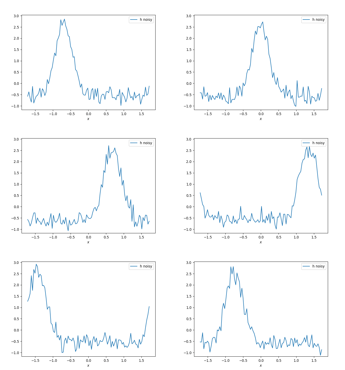
In a real system, we could not expect to immediately have data as smooth as that we used in Section 3. However, the procedure is unchanged. The only challenge will be fitting the neural network to our data. Let’s add some noise to the data:

x,t,noisy_h = load_data("simple_wave.npz",.2)
animation2 = animate_data(x,t,[noisy_h], ["h noisy"])
animation2.save("noisy_h.gif")
plt.close()

Given our data is now noisy, we may want to implement a train-validation-test method for fitting. Simply put, this means that we will hold out a portion of our data from the training procedure. Part of this held-back data (validation set) will be used to validate that our model can generalize to other points during training. The other part of the held-back data (test set) will be used as a final check on how well the model extrapolates out of the training data.

import sklearn.model_selection as ms

X,T = jnp.meshgrid(x,t)
xt_noisy = np.vstack((X.flatten(),T.flatten())).T
h_noisy = noisy_h.flatten()
xt_train, xt_test, h_train, h_test = ms.train_test_split(xt_noisy,h_noisy,test_size=.1,train_size=.9)
xt_train, xt_valid, h_train, h_valid = ms.train_test_split(xt_train,h_train,test_size=.1,train_size=.9)

train_data = batch_data(xt_train[:,0], xt_train[:,1], h_train, 1000)
valid_data = batch_data(xt_valid[:,0], xt_valid[:,1], h_valid, 1000)
test_data = batch_data(xt_test[:,0], xt_test[:,1], h_test, 1000)

Now, we apply our previous model construction and training:

# Initialize model
rng1,rng2 = jax.random.split(jax.random.PRNGKey(42))
random_data = jax.random.normal(rng1,(2,))
model2 = MyNet()
params2 = model2.init(rng2,random_data)

# Loss function
@jax.jit
def mse(params,input,targets):
    def squared_error(x,y):
        pred = model2.apply(params,x)
        return jnp.mean((y - pred)**2)
    return jnp.mean(jax.vmap(squared_error)(input,targets),axis=0)
loss_grad_fn = jax.value_and_grad(mse)

# Optimizer
learning_rate = 1e-2
tx = optax.adam(learning_rate)
opt_state = tx.init(params2)

# Training (adjusted to use our validation data
epochs = 1200
for i in range(epochs):
    xt_batch = train_data[i%len(train_data)][0]
    h_batch = train_data[i%len(train_data)][1]
    loss_val, grads = loss_grad_fn(params2, xt_batch, h_batch)
    updates, opt_state = tx.update(grads, opt_state)
    params2 = optax.apply_updates(params2, updates)
    if i % 100 == 0:
        train_loss = mse(params2,xt_train,h_train)
        valid_loss = mse(params2,xt_valid,h_valid)
        print("Step {}".format(i))
        print("Training loss: {}".format(train_loss))
        print("Validation loss: {}".format(valid_loss))
        print()
test_loss = mse(params2,xt_test,h_test)
print("Test loss after training: {}".format(test_loss))

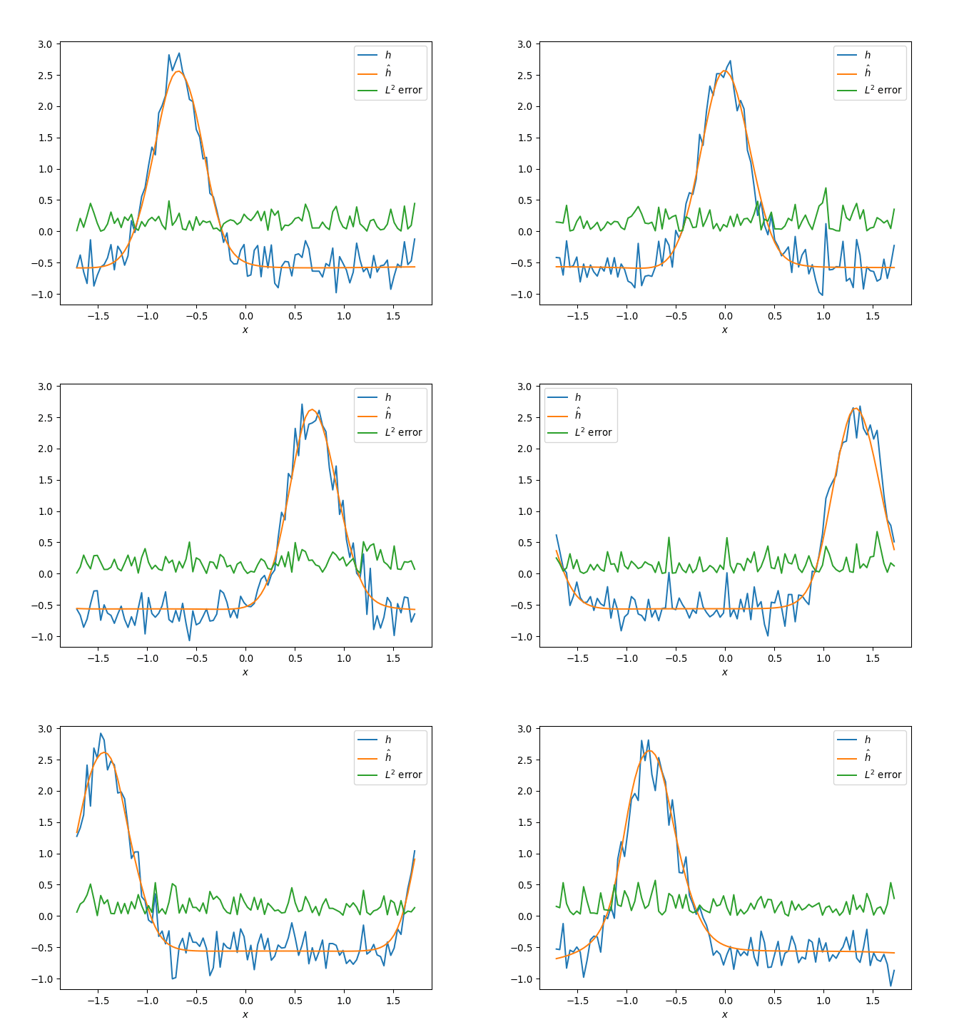
hhat2 = model2.apply(params2,xt_points).reshape(X.shape)
diff = np.sqrt((noisy_h - hhat2)**2)
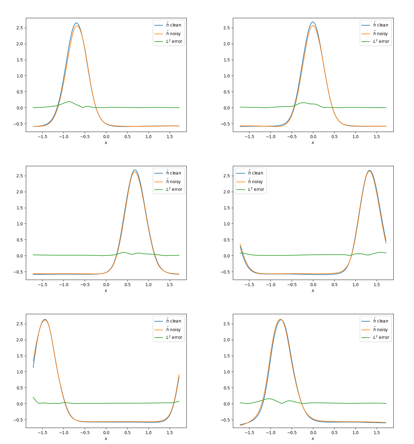
diff2 = np.sqrt((hhat1 - hhat2)**2)
animation3 = animate_data(x,t,[noisy_h,hhat2,diff],["$h$","$\hat{h}$","$L^2$ error"])
animation3.save("noisy_h_compare.gif")
plt.close()
animation3 = animate_data(x,t,[hhat1,hhat2,diff2],["$\hat{h}$ clean","$\hat{h}$ noisy","$L^2$ error"])
animation3.save("noisy_hhat_compare.gif")
plt.close()
Step 0
Training loss: 1.0839306116104126
Validation loss: 1.1880024671554565

Step 100
Training loss: 0.2529764771461487
Validation loss: 0.28380659222602844

Step 200
Training loss: 0.16499020159244537
Validation loss: 0.17510230839252472

Step 300
Training loss: 0.13047386705875397
Validation loss: 0.12965114414691925

Step 400
Training loss: 0.07818066328763962
Validation loss: 0.07242970168590546

Step 500
Training loss: 0.04669160768389702
Validation loss: 0.04420790821313858

Step 600
Training loss: 0.04208264872431755
Validation loss: 0.04083852097392082

Step 700
Training loss: 0.039955753833055496
Validation loss: 0.039250146597623825

Step 800
Training loss: 0.03985001891851425
Validation loss: 0.03994066268205643

Step 900
Training loss: 0.04050833359360695
Validation loss: 0.04085934907197952

Step 1000
Training loss: 0.040248990058898926
Validation loss: 0.040409237146377563

Step 1100
Training loss: 0.0393543541431427
Validation loss: 0.03912331536412239

Test loss after training: 0.039526768028736115

The resulting fit can be seen in the following video:

Looks pretty good all things considered! We can also compare this with the fit on clean data to see how impressive the robustness to noise was:

Finally, we construct the terms and check the results after forward selection:

def model_for_diff(x,t):
    new_x = jnp.array([x,t])
    return model2.apply(params2, new_x)[0]

# Construct terms numerically
diff_term_values = {}
for i in range(max_diff_order+1):
    diff_func = model_for_diff
    # Iteratively apply derivatives
    for _ in range(i):
        diff_func = jax.grad(diff_func, 0)
    def unpack_diff_func(x):
        new_x,new_t = x
        return diff_func(new_x,new_t)
    diff_term_values[diff_terms[i]] = np.array(jax.lax.map(unpack_diff_func, xt_points))
term_values = construct_terms(diff_term_values)

def unpack_diff_func(x):
    new_x,new_t = x
    return jax.grad(model_for_diff,1)(new_x,new_t)

h_t_term = sp.Function("h_t")(x_sym,t_sym)
h_t = -np.array(jax.lax.map(unpack_diff_func, xt_points))

# Forward selection
term_matrix = pd.DataFrame(term_values,index=pd.MultiIndex.from_arrays(np.round(np.array(xt_points),2).T, names=("x","t")))
forward_r2_select(term_matrix, h_t)
R^2: 0.9992922625224863
R^2: 0.9993020536736786
R^2: 0.999314004266004
R^2: 0.9993156257451148
h_x(x, t)
Coefficients 0.999435
h_x(x, t) h_xxx(x, t)**2*h_xxxx(x, t)**2
Coefficients 0.999985 -1.378831e-14
h_x(x, t) h_x(x, t)**3 h_xxx(x, t)**2*h_xxxx(x, t)**2
Coefficients 1.008283 -0.000179 -1.257324e-14
h_x(x, t) h_x(x, t)**3 h_xx(x, t)**2*h_xxxx(x, t)**2 h_xxx(x, t)**2*h_xxxx(x, t)**2
Coefficients 1.009172 -0.000195 -2.579226e-13 -9.285486e-15

Boom! Landed right on the money. This is a simple example with a straightforward answer, but example holds to show the overall procedure for handling data with additive noise (multiplicative noise, which is more structural, would be an altogether different challenge).

Application to extracted wave data

Now, applying this procedure to real data is as simple as replacing our original dataset with an experimental dataset. However, the extraction process has a strong influence on the quality of the data that we will be using, so it deserves to be treated with some detail.

Image data extraction

The original video we will be using can be found on YouTube here.

We can load this video into individual image frames via:

import skimage as img
import imageio.v3 as iio

raw_frames = []
cut = (160,200)
for i in range(200,232):
    frame = iio.imread("youtube_video.mp4",plugin="pyav",index=i)

    # Cut the image to focus only on the wave portion
    raw_frame = frame[cut[0]:cut[1],:,:]
    raw_frames.append(raw_frame)
raw_frames = np.array(raw_frames)
plt.figure(figsize=(8,1))
plt.imshow(raw_frames[16])
plt.axis(False); plt.show()

We then need to remove the background and isolate the wave portion of the image, which is facilitated by the green color of the water in this video:

frames = []
for i in range(len(raw_frames)):
    frame = raw_frames[i]

    # Find where the image is more green than red or blue and very bright green
    mean_green = np.mean(frame[:,:,1])
    std_green = np.std(frame[:,:,1])
    frame = (frame[:,:,1] > frame[:,:,0]) & (frame[:,:,1] > frame[:,:,2]) & (frame[:,:,1] > mean_green+std_green)
    frames.append(frame)
frames = np.array(frames)
plt.figure(figsize=(8,1))
plt.imshow(frames[16],cmap="gray")
plt.axis(False); plt.show()

By averaging these pixels across all vertical pixels in the image, we can get a rough wave outline:

heights = []
for i in range(len(frames)):
    frame = frames[i]
    
    # Approximate wave height by averaging y-locations of bright green areas
    height = np.zeros(frame.shape[1])
    for j in range(frame.shape[1]):
        height[j] = np.mean(np.where(frame[:,j] == 1)[0])
    heights.append(height)
heights = np.array(heights)
base = heights[16, 0]

plt.figure(figsize=(8,1))
plt.imshow(frames[16],cmap="gray")
line = plt.plot(heights[16], color="red",lw=3)[0]
line2 = plt.plot([0,heights.shape[1]], [31,31], color="orange", ls="--")[0]
plt.axis(False); plt.show()

Finally, we can note that the video is not quite level to the wave surface, so we can use a linear adjustment to align the water boundary heights at the middle of the video:

# Adjust images and heights for an un-leveled camera
im_width = len(heights[16])
slope = (heights[16][-1] - heights[16][0]) / im_width
for i in range(len(heights)):
    frame = frames[i]
    height = heights[i]

    # Adjust
    for j in range(len(height)):
        shift = int(slope*(im_width-j))
        # Move frame pixels per column
        frame[:,j] = np.roll(frame[:,j], shift)
        # Move height of wave
        height[j] += shift
    frames[i] = frame
    heights[i] = height

frames = np.array(frames)
raw_frames = np.array(raw_frames)
heights = np.array(heights)

fig = plt.figure(figsize=(8,1))
im = plt.imshow(frames[0],cmap="gray")
line = plt.plot(heights[0], color="red",lw=3)[0]
line2 = plt.plot([0,heights.shape[1]], [31,31], color="orange", ls="--")[0]
plt.axis(False);

def animation_function(i):
    im.set_array(frames[i])
    line.set_ydata(heights[i])
    return [im,line,line2]

wave_animation = anim.FuncAnimation(fig, animation_function, frames=range(len(frames)), blit=True)
wave_animation.save("extracted_wave.gif")
plt.close()

We can now save this data to be used with our previous procedure:

# Video portion is about 2 seconds long
times = np.linspace(0,2,len(heights))
# No given space scale
x_domain = np.arange(len(heights[0]))
np.save("video_wave_images.npy",raw_frames)
np.savez("video_wave_heights.npz",h=heights,x=x_domain,t=times)

Using our experimental dataset

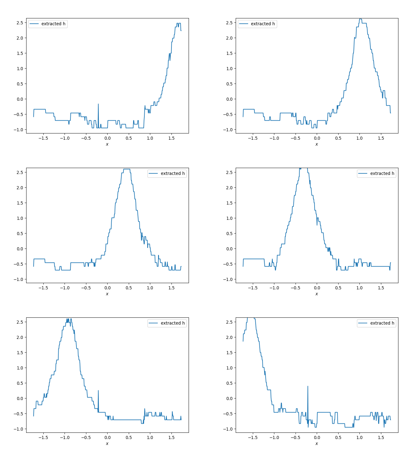
Using the same methods as listed in Section 4, we can discover an equation for this particular dataset:

x,t,ext_h = load_data("video_wave_heights.npz")
# Flip image wave to be more familiar
ext_h = -ext_h
animation2 = animate_data(x,t,[ext_h], ["extracted h"])
animation2.save("extracted_h.gif")
plt.close()

# Splitting data
X,T = jnp.meshgrid(x,t)
xt_ext = np.vstack((X.flatten(),T.flatten())).T
h_ext = ext_h.flatten()
xt_train, xt_test, h_train, h_test = ms.train_test_split(xt_ext,h_ext,test_size=.1,train_size=.9)
xt_train, xt_valid, h_train, h_valid = ms.train_test_split(xt_train,h_train,test_size=.1,train_size=.9)

train_data = batch_data(xt_train[:,0], xt_train[:,1], h_train, 1000)
valid_data = batch_data(xt_valid[:,0], xt_valid[:,1], h_valid, 1000)
test_data = batch_data(xt_test[:,0], xt_test[:,1], h_test, 1000)

# Initialize model
rng1,rng2 = jax.random.split(jax.random.PRNGKey(42))
random_data = jax.random.normal(rng1,(2,))
model3 = MyNet()
params3 = model3.init(rng2,random_data)

# Loss function
@jax.jit
def mse(params,input,targets):
    def squared_error(x,y):
        pred = model3.apply(params,x)
        return jnp.mean((y - pred)**2)
    return jnp.mean(jax.vmap(squared_error)(input,targets),axis=0)
loss_grad_fn = jax.value_and_grad(mse)

# Optimizer
learning_rate = 1e-2
tx = optax.adam(learning_rate)
opt_state = tx.init(params3)

# Training (adjusted to use our validation data
epochs = 1200
for i in range(epochs):
    xt_batch = train_data[i%len(train_data)][0]
    h_batch = train_data[i%len(train_data)][1]
    loss_val, grads = loss_grad_fn(params3, xt_batch, h_batch)
    updates, opt_state = tx.update(grads, opt_state)
    params3 = optax.apply_updates(params3, updates)
    if i % 100 == 0:
        train_loss = mse(params3,xt_train,h_train)
        valid_loss = mse(params3,xt_valid,h_valid)
        print("Step {}".format(i))
        print("Training loss: {}".format(train_loss))
        print("Validation loss: {}".format(valid_loss))
        print()
test_loss = mse(params3,xt_test,h_test)
print("Test loss after training: {}".format(test_loss))

hhat = model3.apply(params3,xt_ext).reshape(X.shape)
diff = np.sqrt((ext_h - hhat)**2)
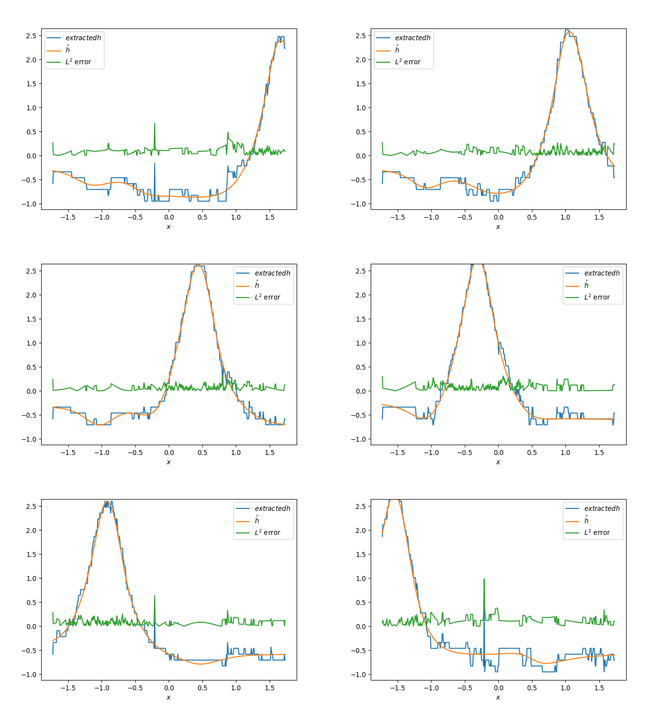
animation3 = animate_data(x,t,[ext_h,hhat,diff],["$extracted h$","$\hat{h}$","$L^2$ error"])
animation3.save("ext_h_compare.gif")
plt.close()
Step 0
Training loss: 1.0430516004562378
Validation loss: 1.0766783952713013

Step 100
Training loss: 0.018125249072909355
Validation loss: 0.01899655908346176

Step 200
Training loss: 0.015589875169098377
Validation loss: 0.016529928892850876

Step 300
Training loss: 0.01496046781539917
Validation loss: 0.01591702178120613

Step 400
Training loss: 0.014640039764344692
Validation loss: 0.015734868124127388

Step 500
Training loss: 0.013847903348505497
Validation loss: 0.015050699934363365

Step 600
Training loss: 0.013422622345387936
Validation loss: 0.0145771699026227

Step 700
Training loss: 0.012840907089412212
Validation loss: 0.014002472162246704

Step 800
Training loss: 0.012728855013847351
Validation loss: 0.01390550285577774

Step 900
Training loss: 0.012514415197074413
Validation loss: 0.013635623268783092

Step 1000
Training loss: 0.011771985329687595
Validation loss: 0.013032175600528717

Step 1100
Training loss: 0.011503455229103565
Validation loss: 0.012660597451031208

Test loss after training: 0.0104597182944417

def model_for_diff(x,t):
    new_x = jnp.array([x,t])
    return model3.apply(params3, new_x)[0]

# Construct terms numerically
diff_term_values = {}
for i in range(max_diff_order+1):
    diff_func = model_for_diff
    # Iteratively apply derivatives
    for _ in range(i):
        diff_func = jax.grad(diff_func, 0)
    def unpack_diff_func(x):
        new_x,new_t = x
        return diff_func(new_x,new_t)
    diff_term_values[diff_terms[i]] = np.array(jax.lax.map(unpack_diff_func, xt_ext))
term_values = construct_terms(diff_term_values)

def unpack_diff_func(x):
    new_x,new_t = x
    return jax.grad(model_for_diff,1)(new_x,new_t)

h_t_term = sp.Function("h_t")(x_sym,t_sym)
h_t = -np.array(jax.lax.map(unpack_diff_func, xt_ext))

# Forward selection
term_matrix = pd.DataFrame(term_values,index=pd.MultiIndex.from_arrays(np.round(np.array(xt_ext),2).T, names=("x","t")))
forward_r2_select(term_matrix, h_t)
R^2: 0.9863934214868251
R^2: 0.9865333532703366
R^2: 0.9882344773693393
R^2: 0.991064364883932
h_x(x, t)
Coefficients -0.965739
h_x(x, t) h_xxx(x, t)
Coefficients -0.97502 -0.000325
h_x(x, t) h_xxx(x, t) h(x, t)*h_xxx(x, t)
Coefficients -0.967936 -0.003446 0.001618
h_x(x, t) h_xxx(x, t) h(x, t)*h_xxx(x, t) h(x, t)**2*h_xxx(x, t)
Coefficients -0.943376 -0.006432 0.00772 -0.002068

Feel free to play with the parameters of each step to try to change/improve the results we have seen here.

Appendix

The benefits of JAX

jax is an automatic differentiation based on the XLA compiler for Tensorflow. The largest difference between this library and the alternative libraries (like those included in tensorflow main, pytorch, keras, etc.) is that it compiles Python code down to a computational graph structure. Although the majority of excitement around this compiler has surrounded the optimizations that can take place one the graph structure has been identified, it also facilitates taking derivatives of arbitrarry objects. This is because rather than compute gradients along the path (forward mode automatic differentiation) or keeping track of operations as it goes (backward mode automatic differentiation), it has a graph structure to analyze exactly what happens to each value and parameter. At the end of the day, this means it is much easier to compute gradients of exactly what you want.

If jax and flax have appeared too hands-on and complicated after this workshop, consider trying treex which aims to make using jax for neural networks simple and only need a few lines of code.

Training without normalizing the data

In the Section 3 section, the load_data function performs a normalization of the simulated data from a range of \(h(x,t) \in [0,.1]\) where \(x \in [0,1]\) and \(t \in [0,1]\) to a range of \(h(x,t) \in [-1,1]\) with mean \(\bar{h}=0\) and standard deviation 1 with \(x \in [-1.7,1.7]\) and \(t \in [-1.7,1.7]\). Normalizing data like this is common in machine learning, but it is not always apparent why. Our case can give a strong demonstration as to the benefits of normalizing in this way.

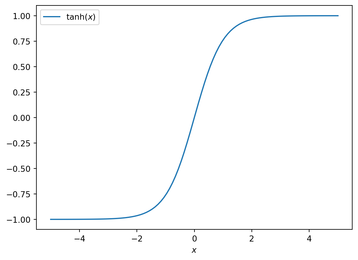
Consider that our neural network uses only the \(\tanh\) activation function. For those unfamiliar, this function has the form:

tanh_dom = np.linspace(-5,5,100)
tanh_range = np.tanh(tanh_dom)
plt.plot(tanh_dom, tanh_range, label="$\\tanh(x)$")
plt.xlabel("$x$"); plt.legend(); plt.show()

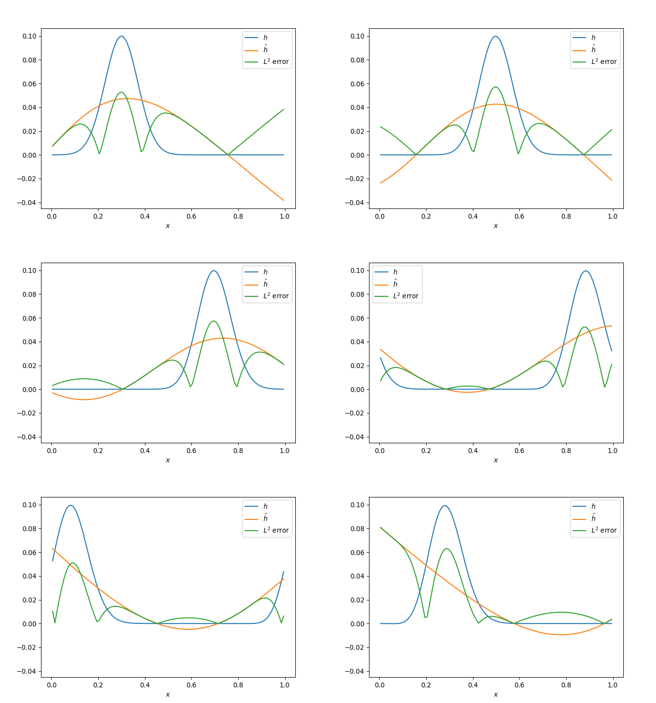
Each layer of our neural network is connected via linear transformations of the form \(\vec{x}^T\mathbf{W} + \vec{b}\), thus we should be able to shift the data into the appropriate domain and range for the \(\tanh\) function. However, in practice, optimizing our parameters to attain this is hard to find. To demonstrate, consider the training of the neural network on clean simulation data without normalization:

x,t,h = load_data("simple_wave.npz",norm=False)
X,T = jnp.meshgrid(x,t)
data = batch_data(X.flatten(),T.flatten(),h.flatten(),10000)
# Random generator seed
rng1,rng2 = jax.random.split(jax.random.PRNGKey(42))
random_data = jax.random.normal(rng1,(2,))
model4 = MyNet()
params4 = model1.init(rng2,random_data)

@jax.jit
def mse(params,input,targets):
    def squared_error(x,y):
        pred = model4.apply(params,x)
        return jnp.mean((y - pred)**2)
    return jnp.mean(jax.vmap(squared_error)(input,targets),axis=0)
loss_grad_fn = jax.value_and_grad(mse)

learning_rate = 1e-2
tx = optax.adam(learning_rate)
opt_state = tx.init(params4)

epochs = 1000
all_xt = jnp.array([data[i][0] for i in range(len(data))])
all_h = jnp.array([data[i][1] for i in range(len(data))])
for i in range(epochs):
    xt_batch = data[i%len(data)][0]
    h_batch = data[i%len(data)][1]
    loss_val, grads = loss_grad_fn(params4, xt_batch, h_batch)
    updates, opt_state = tx.update(grads, opt_state)
    params4 = optax.apply_updates(params4, updates)
    if i % 100 == 0:
        train_loss = mse(params4,all_xt,all_h)
        print("Training loss step {}: {}".format(i,train_loss))

xt_points = jnp.vstack([X.flatten(),T.flatten()]).T
hhat4 = model1.apply(params4,xt_points).reshape(X.shape)
diff = np.sqrt((h - hhat4)**2)
animation4 = animate_data(x,t,[h,hhat4,diff],["$h$","$\hat{h}$","$L^2$ error"])
animation4.save("nonorm_h_compare.gif")
plt.close()
Training loss step 0: 0.3563382923603058
Training loss step 100: 0.0009187606628984213
Training loss step 200: 0.0008465295541100204
Training loss step 300: 0.0007735079852864146
Training loss step 400: 0.0006919147563166916
Training loss step 500: 0.0006207430851645768
Training loss step 600: 0.0005757115432061255
Training loss step 700: 0.0005529409390874207
Training loss step 800: 0.0005375399487093091
Training loss step 900: 0.0005216019926592708

The fit is terrible! We have apparently fallen into a local minimum far from the global minimum we would like to find. This demonstrates two important ideas relating to neural networks (validated by experience):

  1. They are fickle and in some cases small changes to data, architecture, and training, can dramatically change results
  2. Any help that can be given to the neural network via knowledge of the system or data can help. In this case, adjusting for the gap between the range of our data and that of the activation function was sufficient.

References

[1]
S. L. Brunton, J. L. Proctor, and J. N. Kutz, Discovering Governing Equations from Data by Sparse Identification of Nonlinear Dynamical Systems, Proceedings of the National Academy of Sciences 113, 3932 (2016).
[2]
M. O. Williams, I. G. Kevrekidis, and C. W. Rowley, A Data–Driven Approximation of the Koopman Operator: Extending Dynamic Mode Decomposition, Journal of Nonlinear Science 25, 1307 (2015).
[3]
W. S. Cleveland and S. J. Devlin, Locally Weighted Regression: An Approach to Regression Analysis by Local Fitting, Journal of the American Statistical Association 83, 596 (1988).
[4]
W. H. Press and S. A. Teukolsky, Savitzky-Golay Smoothing Filters, Computers in Physics 4, 669 (1990).
[5]
P. Zheng, T. Askham, S. L. Brunton, J. N. Kutz, and A. Y. Aravkin, A Unified Framework for Sparse Relaxed Regularized Regression: SR3, IEEE Access 7, 1404 (2018).
[6]
S. H. Rudy, S. L. Brunton, J. L. Proctor, and J. N. Kutz, Data-Driven Discovery of Partial Differential Equations, Science Advances 3, e1602614 (2017).
[7]
H. Xu, H. Chang, and D. Zhang, Dl-Pde: Deep-Learning Based Data-Driven Discovery of Partial Differential Equations from Discrete and Noisy Data, arXiv Preprint arXiv:1908.04463 (2019).