import gymnasium as gym
import random
import numpy as np
from IPython.display import Image
import matplotlib.pyplot as plt❄️ Frozen Lake
Frozen Lake is a simple environment composed of tiles, where the AI has to move from an initial tile to a goal.
Tiles can be a safe frozen lake ✅, or a hole ❌ that gets you stuck forever.
The AI, or agent, has 4 possible actions: go ◀️ LEFT, 🔽 DOWN, ▶️ RIGHT, or 🔼 UP.
The agent must learn to avoid holes in order to reach the goal in a minimal number of actions.
Required Libraries
Initialize the Environment
env = gym.make("FrozenLake-v1", is_slippery = False) #in non-slippery version actions cannot be ignored
env.reset()
env.render()
/Users/cjrobe/miniforge3/envs/website/lib/python3.11/site-packages/gymnasium/envs/toy_text/frozen_lake.py:328: UserWarning: WARN: You are calling render method without specifying any render mode. You can specify the render_mode at initialization, e.g. gym.make("FrozenLake-v1", render_mode="rgb_array")
gym.logger.warn(- S: starting point, safe
- F: frozen surface, safe
- H: hole, stuck forever
- G: goal, safe
Image(filename = "FrozenLake.gif", width=400)<IPython.core.display.Image object>Image(filename = "Final.gif", width=400)<IPython.core.display.Image object>Reward
Reward schedule:
Reach goal(G): +1
Reach hole(H): 0
Reach frozen surface(F): 0
Size of Action and State Space
print("State space: ", env.observation_space.n)
print("Action space: ", env.action_space.n)
State space: 16
Action space: 4In Frozen Lake, there are 16 tiles, which means our agent can be found in 16 different positions, called states.
For each state, there are 4 possible actions:
- ◀️ LEFT: 0
- 🔽 DOWN: 1
- ▶️ RIGHT: 2
- 🔼 UP: 3
Initialize Q Table
Image(filename = "QTable.gif", width=400)<IPython.core.display.Image object># Our table has the following dimensions:
# (rows x columns) = (states x actions) = (16 x 4)
nb_states = env.observation_space.n # = 16
nb_actions = env.action_space.n # = 4
qtable = np.zeros((nb_states, nb_actions))
# Let's see how it looks
print('Q-table =')
print(qtable)Q-table =
[[0. 0. 0. 0.]
[0. 0. 0. 0.]
[0. 0. 0. 0.]
[0. 0. 0. 0.]
[0. 0. 0. 0.]
[0. 0. 0. 0.]
[0. 0. 0. 0.]
[0. 0. 0. 0.]
[0. 0. 0. 0.]
[0. 0. 0. 0.]
[0. 0. 0. 0.]
[0. 0. 0. 0.]
[0. 0. 0. 0.]
[0. 0. 0. 0.]
[0. 0. 0. 0.]
[0. 0. 0. 0.]]Update Formula
$ Q_{new}(s_t, a_t) = Q(s_t, a_t) + (r_t + max_a Q(s_{t+1}, a) - Q(s_t, a_t)) $
Epsilon-Greedy Algorithm
In this method, we want to allow our agent to either:
- Take the action with the highest value (exploitation);
- Choose a random action to try to find even better ones (exploration).
Image(filename = "tradeoff.gif", width=700)<IPython.core.display.Image object>Hyperparameters
episodes = 1000        # Total number of episodes
alpha = 0.5            # Learning rate
gamma = 0.9            # Discount factor
epsilon = 1.0          # Amount of randomness in the action selection
epsilon_decay = 0.001  # Fixed amount to decrease
Training
# List of outcomes to plot
outcomes = []

for _ in range(episodes):

    state,info = env.reset()
    done = False

    # By default, we consider our outcome to be a failure
    outcomes.append("Failure")

    # Until the agent gets stuck in a hole or reaches the goal, keep training it
    while not done:
        # Generate a random number between 0 and 1
        rnd = np.random.random()

        # If random number < epsilon, take a random action
        if rnd < epsilon:
            action = env.action_space.sample()
        # Else, take the action with the highest value in the current state
        else:
            action = np.argmax(qtable[state])

        # Implement this action and move the agent in the desired direction
        new_state, reward, done, _, info = env.step(action)

        # Update Q(s,a)
        qtable[state, action] = qtable[state, action] + \
                                alpha * (reward + gamma * np.max(qtable[new_state]) - qtable[state, action])

        # Update our current state
        state = new_state

        # If we have a reward, it means that our outcome is a success
        if reward:
            outcomes[-1] = "Success"

    # Update epsilon
    epsilon = max(epsilon - epsilon_decay, 0)
Updated Q Table
print('===========================================')
print('Q-table after training:')
print(qtable)
===========================================
Q-table after training:
[[0.531441 0.59049 0.59048919 0.531441 ]
[0.531441 0. 0.65609983 0.56212481]
[0.50422703 0.72899998 0.12149802 0.61759207]
[0.45242846 0. 0. 0. ]
[0.59049 0.6561 0. 0.531441 ]
[0. 0. 0. 0. ]
[0. 0.81 0. 0.60486928]
[0. 0. 0. 0. ]
[0.6561 0. 0.729 0.59049 ]
[0.6561 0.81 0.81 0. ]
[0.72894994 0.9 0. 0.72001722]
[0. 0. 0. 0. ]
[0. 0. 0. 0. ]
[0. 0.81 0.9 0.729 ]
[0.81 0.9 1. 0.81 ]
[0. 0. 0. 0. ]]Plot Outcomes
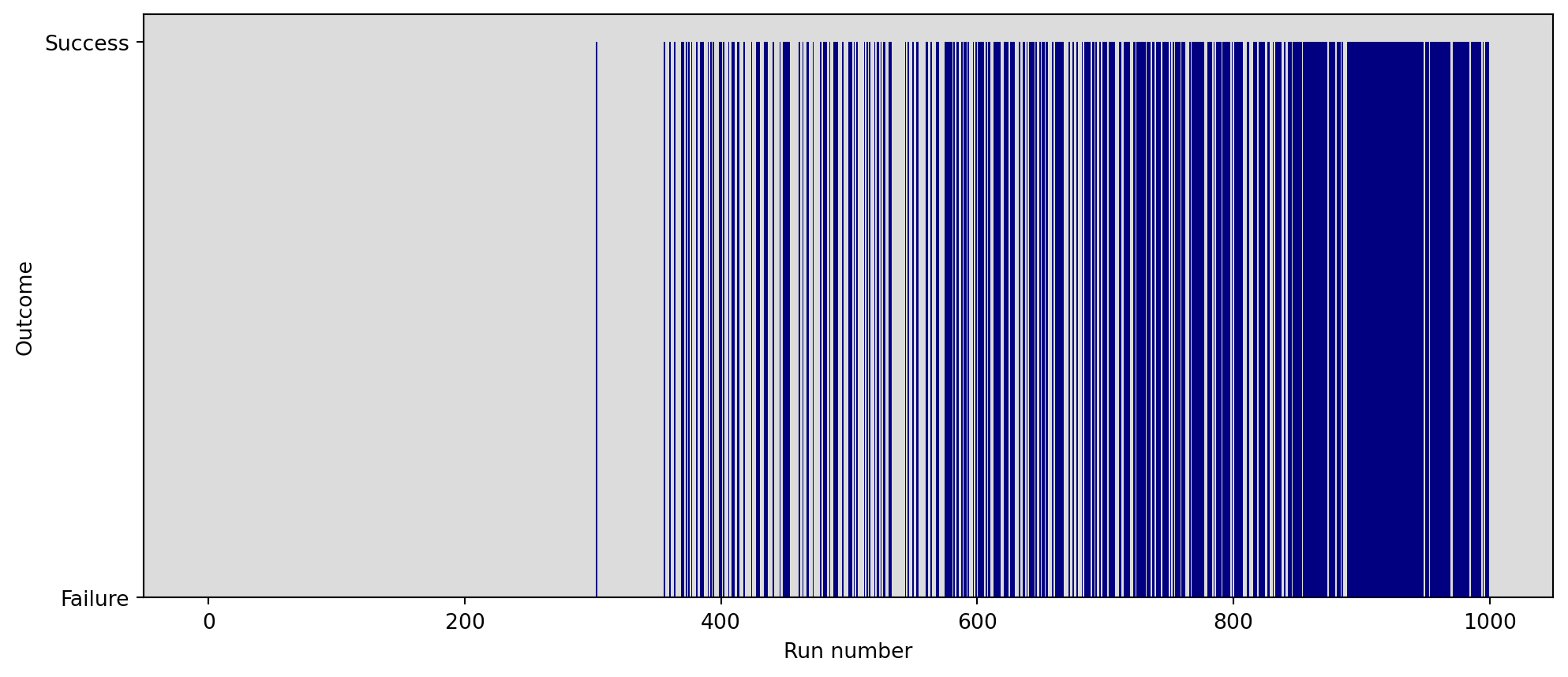
plt.figure(figsize=(12, 5))
plt.xlabel("Run number")
plt.ylabel("Outcome")
ax = plt.gca()
ax.set_facecolor('gainsboro')
plt.bar(range(len(outcomes)), outcomes, color="navy", width=1.0)
plt.show()
Evaluation
episodes = 1
nb_success = 0


state,info = env.reset()
env.render()
done = False

# Until the agent gets stuck or reaches the goal, keep training it
while not done:

    # Choose the action with the highest value in the current state
    action = np.argmax(qtable[state])

    # Implement this action and move the agent in the desired direction
    new_state, reward, done, _, info = env.step(action)

    # Render the environment
    print()
    env.render()

    # Update our current state
    state = new_state

    # When we get a reward, it means we solved the game
    nb_success += reward

# Let's check our success rate!
print()
print (f"Success rate = {nb_success/episodes*100}%")
Success rate = 100.0%