Lab 3 - Fixed point methods
Introduction
Our goal is to find the fixed point of a function \(g(x)\), that is, the value \(x^*\) such that \(x^*= g(x^*)\) (if it exists). If \(|g'(x^{*})|<1\), we can find the fixed point by iteration if we start sufficiently close to \(x^*\).
For the example problem \(g(x) = \cos{(x)}\), we can begin with an initial guess \(x_1=0.5\) and find the next point, \(x_2\), by applying \(g\): \(x_2=g(x_1)\). We repeat this process \(n\) times to find \(x_{n+1}=g(x_n)\). This can be summarized in the following table:
| n | $ x_n$ | $x_{n+1}=(x_n) $ | $ E_n= |
|---|---|---|---|
| 1 | 0.5000 | 0.8775 | 0.3775 |
| 2 | 0.8775 | 0.6390 | 0.2385 |
| 3 | 0.6390 | 0.8026 | 0.1636 |
| 4 | 0.8026 | 0.6947 | 0.1079 |
| 5 | 0.6947 | 0.7681 | 0.0734 |
| 6 | 0.7681 | 0.7191 | 0.0490 |
| 7 | 0.7191 | 0.7523 | 0.0331 |
| 8 | 0.7523 | 0.7300 | 0.0222 |
| 9 | 0.7300 | 0.7451 | 0.0150 |
| 10 | 0.7451 | 0.7350 | 0.0101 |
| 11 | 0.7350 | 0.7418 | 0.0068 |
This table shows an iteration \(n\), the \(x\) value \(x_n\), the result of the iteration \(x_{n+1} = \cos(x_n)\), and the difference between the current step and the next \(E_n = |x_n - x_{n+1}|\). Note that the difference in \(x_i\) between each step gets smaller and smaller as we iterate. This shows that we are indeed approaching a fixed point. In this case, if we continue we will eventually converge to the fixed point \(x^*\approx0.739085133\).
This process is only guaranteed to converge if \(|g'(x^*)|<1\). In this case, \(g(x)\) is “contracting” around \(x^*\). To see this contraction visually, we can consider the following image:
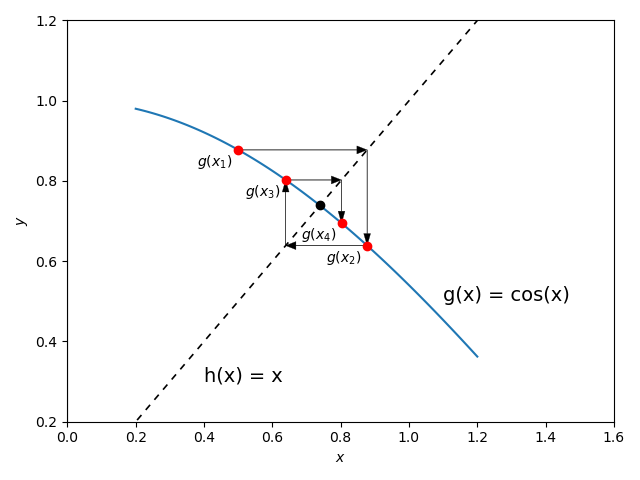
In this image, the dashed line represents the line \(y=x\), so the arrows go from \((x_1, g(x_1))\to (x_2, x_2) \to (x_2, g(x_2)) \to \ldots (x_4, g(x_4)\).
In practice, we do not know when we have arrived at the fixed point \(x^*\), so we instead stop by looking at the difference between iterations: \(E_n = |x_{n+1} - x_n|\). When this difference becomes sufficiently small, we can assume that we have the best answer that the fixed point method can give us.
Below is a program that performs fixed point iteration for a given function \(g(x)\). The convergence criterion for the program will be given by the error condition which can be written as: \[ \begin{align*} E_n={|x_{n+1} - x_n|} <\text{ tol} \end{align*} \] where tol is a given tolerance.
Although \(|g'(x^*)|<1\) guarantees that the method will converge , in practice we usually do not know the interval. Thus, if your initial guess for \(x^*\) is not sufficiently close to the actual value of \(x^*\) the method may not converge. Informed initial guesses and trial and error are common techniques for overcoming this shortcoming.
Newton’s Method
Newton’s method is a fixed point iteration that converges to the root of a function \(f(x)\). It uses the iteration function: \[ \begin{align*} g(x) = x - \frac{f(x)}{f'(x)} .\end{align*} \] Analyzing this function, we can see that the fixed point \(x^*\) for \(g(x)\) is also the root of \(f(x)\): \[ \begin{align*} g(x^*) &= x^{*} \\ x^* - \frac{f(x^*)}{f'(x^*)}&= x^* \\ - \frac{f(x^*)}{f'(x^*)} &= 0 \\ f(x^*) &= 0 \end{align*} \] as long as \(f'(x^*) \neq 0\).
Convergence
This method was published in 1685 but is still one of the state-of-the-art methods for root finding because it “converges” so quickly. The idea of convergence is key to numerical methods and refers to the rate at which the error decreases as you perform more iterations. The easiest way to illustrate convergence is to consider the Taylor series of our fixed point iteration centered at \(x^*\): \[ \begin{align*} g(x_{n}) &= g(x^*) + g'(c)(x_{n}-x^*) \end{align*} \] for some \(c \in (x^*, x_{n})\). We can then substitute \(g(x_{n}) = x_{n+1}\) and rearrange to get: \[ \begin{align*} g(x_{n}) &= g(x^*) + g'(c)(x_{n}-x^*) \\ x_{n+1} &= x^* + g'(c)(x_{n} - x^*) \\ \frac{x_{n+1} - x^*}{x_{n}-x^*} &= g'(c)\\ \frac{|x_{n+1} - x^*|}{|x_{n}-x^*|} &= |g'(c)| < 1\\ \end{align*} \] as long as \(c\) is close enough to \(x^*\). Thus, we know that \(|x_n - x^*|\) is larger than \(|x_{n+1} - x^*|\) which means we are getting closer and closer to the fixed point with each iteration. We also know that the error at step \(n+1\) over the error at step \(n\) is some constant \(g'(c)\). If \(g'(c) \neq 0\) and \(g'(c) < 1\), then this is called “first-order” convergence. This means, for example, if our error at step \(n\) is \(\frac{1}{2}\) and our constant is \(1\), our error will be reduced by \(\frac{1}{2}\) after 1 step.
However, if our fixed point iteration has the property that \(g'(x^*) = 0\), then we have to take a higher-order Taylor series: \[ \begin{align*} g(x_{n}) &= g(x^*) + g'(x^*)(x_{n}-x^*) +\frac{1}{2} g"(c)(x_{n}-x^*)^2 \\ x_{n+1} &= x^* + \frac{1}{2} g"(c)(x_{n}-x^*)^2 \\ \frac{x_{n+1} - x^*}{(x_n - x^*)^2} &= \frac{1}{2} g"(c) \\ \frac{|x_{n+1} - x^*|}{|x_n - x^*|^2} &= \frac{1}{2} |g"(c)| = C .\end{align*} \] Now, the error at step \(n+1\) over the SQUARE of the error at the previous step is equal to a constant. This is called “second-order” convergence. This means, for example, if our error at step \(n\) is \(\frac{1}{2}\) and the constant is \(1\), then our error will be reduced by \(\frac{1}{2}^{2} = \frac{1}{4}\) after 1 step. Thus, it will take far fewer iterations to converge on the true answer. Newton’s method is a “second-order” method.
One way to test this convergence is by assuming we are near the fixed point and considering: \[ \begin{align*} E_n = |x_{n} - x_{n-1}| \end{align*} \] then we can write the convergence definition approximately as: \[ \begin{align*} C = \frac{|x_{n+1} - x^*|}{|x_n - x^*|^d} &\approx \frac{|x_{n+1} - x_n|}{|x_n - x_{n-1}|^d} \\ &= \frac{E_n}{(E_{n-1})^d} \end{align*} \] where \(C\) is some constant and \(d\) is our order of convergence. This approximation really only makes sense when \(x_n\) and \(x_{n-1}\) are close to \(x^*\). However, we can check this version numerically by computing the error \(E_n\) of our method and then trying \(\frac{E_n}{E_{n-1}^d}\) with different values of \(d\) to see which one is roughly constant.
Examples
The following is a Matlab function that takes in a contraction function \(g\), a starting value \(x_1\), and an error tolerance . It outputs an array that contains all your iteration values: \(x = [x_1, x_2, x_3, \ldots, x_N]\). The convergence criteria for the function is the error: \(|x_{n+1} - x_n| < \text{tol}\).
%| output: false
%%file MyFixedPoint.m
function [xs] = MyFixedPoint(g, x1, tol)
    xs = [x1];
    err = Inf;
    while err > tol
        xs = [xs g(xs(end))];
        err = abs(xs(end) - xs(end-1));
    end
end
Testing this function on \(g(x) = \sin(x-5)\) with starting point \(x_1 = 1\) and a tolerance of \(10^{-7}\) is close to \(0.847\):
g = @(x) sin(x - 5);
p1 = MyFixedPoint(g, 1, 1e-7);
p1(end)
Newton’s method
Consider finding the root of the function \(f(x) = x - \cos(x) - 1\). To find the root of this function with Newton’s method, we need to reformulate it as a fixed point problem in which the fixed point is the root. This can be easily done by considering: \[ \begin{align*} f'(x) &= 1 + sin(x) \\ g(x) &= x - \frac{f(x)}{f'(x)} \\ &= x - \frac{x - \cos(x) -1 }{1 + \sin(x)} \end{align*} \] To approximate the root of the function with an initial guess of \(x_1 = 2.5\) and a tolerance of \(10^{-10}\):
g = @(x) x - ((x - 1 - cos(x))/ (1 + sin(x)));
[xVec] = MyFixedPoint(@(x)g(x), 2.5, 1e-10);
errorVec = [0 abs(xVec(2:end) - xVec(1:end-1))];
nVec=1:1:length(xVec);
p2_table = table(transpose(nVec), transpose(xVec), transpose(errorVec));
p2_table.Properties.VariableNames=["n", "x_n", "E_n"]; disp(p2_table);
If we make a table with the ratios \(\frac{E_n}{E_{n-1}}\), \(\frac{E_n}{(E_{n-1})^2}\), and \(\frac{E_n}{(E_{n-1})^3}\) the preivous results, we can examine an approximate convergence rate for the method:
errorVec = [0 abs(xVec(2:end) - xVec(1:end-1))];
ratio1 = errorVec(2:end) ./ errorVec(1:end-1);
ratio2 = errorVec(2:end) ./ (errorVec(1:end-1) .^2);
ratio3 = errorVec(2:end) ./ (errorVec(1:end-1) .^3);
p2_table = table(ratio1', ratio2', ratio3');
p2_table.Properties.VariableNames=["E_n / E_n-1", "E_n / E_n-1^2", "E_n / E_n-1^3"];
disp(p2_table);
In this, we can see that the second column (which represents a roughly quadratic convergence) is roughly constant, demonstrating that this ratio is holding true. On the other hand, the first column decays to 0, showing that the errors
Stability of fixed points
Consider the function \(g(x) = 1.8x - x^2\) which has fixed points \(x=0\) and \(x=0.8\). If we use an initial guess \(x_1 = 0.1\) and tolerance \(10^{-5}\):
g = @(x) 1.8*x - x^2;
p3 = MyFixedPoint(g, .1, 1e-5);
disp(p3(end))
We approach the fixed point \(x=0.8\) because it is a stable (attracting) fixed point. On the other hand, if we start at \(x_1 = -0.1\):
g = @(x) 1.8*x - x^2;
p3 = MyFixedPoint(g, -0.1, 1e-5);
disp(['Final answer: ', num2str(p3(end))])
We are no longer in the basin of attraction of \(x=0.8\) and so our iteration is expelled from the unstable fixed point \(x=0\).